Main Content

nyquistoptions

Create list of Nyquist plot options

Description

Use the nyquistoptions command to create a NyquistPlotOptions object to customize your Nyquist plot appearance. You can also use the command to override the plot preference settings in the MATLAB® session in which you create the Nyquist plots.

Creation

Description

example

plotoptions = nyquistoptions returns a default set of plot options for use with the nyquistplot command. You can use these options to customize the Nyquist plot appearance using the command line. This syntax is useful when you want to write a script to generate plots that look the same regardless of the preference settings of the MATLAB session in which you run the script.

example

plotoptions = nyquistoptions('cstprefs') initializes the plot options with the options you selected in the Control System Toolbox™ and System Identification Toolbox™ Preferences Editor. For more information about the editor, see Toolbox Preferences Editor. This syntax is useful when you want to change a few plot options but otherwise use your default preferences. A script that uses this syntax may generate results that look different when run in a session with different preferences.

Properties

expand all

Frequency units, specified as one of the following values:

  • 'Hz'

  • 'rad/s'

  • 'rpm'

  • 'kHz'

  • 'MHz'

  • 'GHz'

  • 'rad/nanosecond'

  • 'rad/microsecond'

  • 'rad/millisecond'

  • 'rad/minute'

  • 'rad/hour'

  • 'rad/day'

  • 'rad/week'

  • 'rad/month'

  • 'rad/year'

  • 'cycles/nanosecond'

  • 'cycles/microsecond'

  • 'cycles/millisecond'

  • 'cycles/hour'

  • 'cycles/day'

  • 'cycles/week'

  • 'cycles/month'

  • 'cycles/year'

Magnitude units, specified as either 'dB' or absolute value 'abs'.

Phase units, specified as either 'deg' or 'rad' to change to degrees or radians, respectively.

Toggle display of the response for negative frequencies, specified as either 'on' or 'off'.

Number of standard deviations to use to plot the confidence region, specified as a scalar. This is applicable to identified models only.

Frequency spacing of the confidence ellipses to use to plot the confidence region, specified as a scalar. This is applicable to identified models only. The default value is 5, which means the confidence ellipses are shown at every 5th frequency sample.

Grouping of input-output (I/O) pairs, specified as one of the following:

  • 'none' — No input-output grouping.

  • 'inputs' — Group only the inputs.

  • 'outputs' — Group only the outputs.

  • 'all' — Group all the I/O pairs.

Input label style, specified as a structure with the following fields:

  • FontSize — Font size, specified as a scalar value greater than zero in point units. The default font size depends on the specific operating system and locale. One point equals 1/72 inch.

  • FontWeight — Character thickness, specified as 'Normal' or 'bold'. MATLAB uses the FontWeight property to select a font from those available on your system. Not all fonts have a bold weight. Therefore, specifying a bold font weight can still result in the normal font weight.

  • FontAngle — Character slant, specified as 'Normal' or 'italic'. Not all fonts have both font styles. Therefore, the italic font might look the same as the normal font.

  • Color — Text color, specified as an RGB triplet. The default color is dark grey with the RGB triplet [0.4,0.4,0.4].

  • Interpreter — Text interpreter, specified as one of these values:

    • 'tex' — Interpret characters using a subset of TeX markup. This is the default value of Interpreter.

    • 'latex' — Interpret characters using LaTeX markup.

    • 'none' — Display literal characters.

Output label style, specified as a structure with the following fields:

  • FontSize — Font size, specified as a scalar value greater than zero in point units. The default font size depends on the specific operating system and locale. One point equals 1/72 inch.

  • FontWeight — Character thickness, specified as 'Normal' or 'bold'. MATLAB uses the FontWeight property to select a font from those available on your system. Not all fonts have a bold weight. Therefore, specifying a bold font weight can still result in the normal font weight.

  • FontAngle — Character slant, specified as 'Normal' or 'italic'. Not all fonts have both font styles. Therefore, the italic font might look the same as the normal font.

  • Color — Text color, specified as an RGB triplet. The default color is dark grey with the RGB triplet [0.4,0.4,0.4].

  • Interpreter — Text interpreter, specified as one of these values:

    • 'tex' — Interpret characters using a subset of TeX markup. This is the default value of Interpreter.

    • 'latex' — Interpret characters using LaTeX markup.

    • 'none' — Display literal characters.

Toggle display of inputs, specified as either {'on'}, {'off'} or a cell array with multiple elements.

Toggle display of outputs, specified as either {'on'}, {'off'} or a cell array with multiple elements.

Title text and style, specified as a structure with the following fields:

  • String — Label text, specified as a character vector. By default, the plot is titled 'Nyquist Diagram'.

  • FontSize — Font size, specified as a scalar value greater than zero in point units. The default font size depends on the specific operating system and locale. One point equals 1/72 inch.

  • FontWeight — Character thickness, specified as 'Normal' or 'bold'. MATLAB uses the FontWeight property to select a font from those available on your system. Not all fonts have a bold weight. Therefore, specifying a bold font weight can still result in the normal font weight.

  • FontAngle — Character slant, specified as 'Normal' or 'italic'. Not all fonts have both font styles. Therefore, the italic font might look the same as the normal font.

  • Color — Text color, specified as an RGB triplet. The default color is black specified by the RGB triplet [0,0,0].

  • Interpreter — Text interpreter, specified as one of these values:

    • 'tex' — Interpret characters using a subset of TeX markup. This is the default value of Interpreter.

    • 'latex' — Interpret characters using LaTeX markup.

    • 'none' — Display literal characters.

X-axis label text and style, specified as a structure with the following fields:

  • String — Label text, specified as a character vector. By default, the axis is titled 'Real Axis'.

  • FontSize — Font size, specified as a scalar value greater than zero in point units. The default font size depends on the specific operating system and locale. One point equals 1/72 inch.

  • FontWeight — Character thickness, specified as 'Normal' or 'bold'. MATLAB uses the FontWeight property to select a font from those available on your system. Not all fonts have a bold weight. Therefore, specifying a bold font weight can still result in the normal font weight.

  • FontAngle — Character slant, specified as 'Normal' or 'italic'. Not all fonts have both font styles. Therefore, the italic font might look the same as the normal font.

  • Color — Text color, specified as an RGB triplet. The default color is black specified by the RGB triplet [0,0,0].

  • Interpreter — Text interpreter, specified as one of these values:

    • 'tex' — Interpret characters using a subset of TeX markup. This is the default value of Interpreter.

    • 'latex' — Interpret characters using LaTeX markup.

    • 'none' — Display literal characters.

Y-axis label text and style, specified as a structure with the following fields:

  • String — Label text, specified as a cell array of character vectors. By default, the axis is titled 'Imaginary Axis'.

  • FontSize — Font size, specified as a scalar value greater than zero in point units. The default font size depends on the specific operating system and locale. One point equals 1/72 inch.

  • FontWeight — Character thickness, specified as 'Normal' or 'bold'. MATLAB uses the FontWeight property to select a font from those available on your system. Not all fonts have a bold weight. Therefore, specifying a bold font weight can still result in the normal font weight.

  • FontAngle — Character slant, specified as 'Normal' or 'italic'. Not all fonts have both font styles. Therefore, the italic font might look the same as the normal font.

  • Color — Text color, specified as an RGB triplet. The default color is black specified by the RGB triplet [0,0,0].

  • Interpreter — Text interpreter, specified as one of these values:

    • 'tex' — Interpret characters using a subset of TeX markup. This is the default value of Interpreter.

    • 'latex' — Interpret characters using LaTeX markup.

    • 'none' — Display literal characters.

Tick label style, specified as a structure with the following fields:

  • FontSize — Font size, specified as a scalar value greater than zero in point units. The default font size depends on the specific operating system and locale. One point equals 1/72 inch.

  • FontWeight — Character thickness, specified as 'Normal' or 'bold'. MATLAB uses the FontWeight property to select a font from those available on your system. Not all fonts have a bold weight. Therefore, specifying a bold font weight can still result in the normal font weight.

  • FontAngle — Character slant, specified as 'Normal' or 'italic'. Not all fonts have both font styles. Therefore, the italic font might look the same as the normal font.

  • Color — Text color, specified as an RGB triplet. The default color is black specified by the RGB triplet [0,0,0].

Toggle grid display on the plot, specified as either 'off' or 'on'.

Color of the grid lines, specified as an RGB triplet. The default color is light grey specified by the RGB triplet [0.15,0.15,0.15].

Selection mode for the x-axis limits, specified as one of these values:

  • 'auto' — Enable automatic limit selection, which is based on the total span of the plotted data.

  • 'manual' — Manually specify the axis limits. To specify the axis limits, set the XLim property.

Selection mode for the y-axis limits, specified as one of these values:

  • 'auto' — Enable automatic limit selection, which is based on the total span of the plotted data.

  • 'manual' — Manually specify the axis limits. To specify the axis limits, set the YLim property.

X-axis limits, specified as a cell array of two-element vector of the form [min,max].

Y-axis limits, specified as a cell array of two-element vector of the form [min,max].

Object Functions

nyquistplotNyquist plot with additional plot customization options

Examples

collapse all

For this example, use the plot handle to change the phase units to radians and to turn the grid on.

Generate a random state-space model with 5 states and create the Nyquist diagram with plot handle h.

rng("default")
sys = rss(5);
h = nyquistplot(sys);

Figure contains an axes object. The axes object contains an object of type line. This object represents sys.

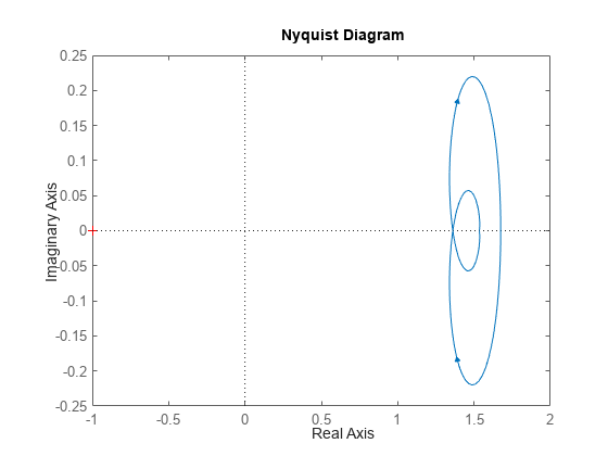
Change the phase units to radians and turn on the grid. To do so, edit properties of the plot handle, h using setoptions.

setoptions(h,'PhaseUnits','rad','Grid','on');

Figure contains an axes object. The axes object contains an object of type line. This object represents sys.

The Nyquist plot automatically updates when you call setoptions.

Alternatively, you can also use the nyquistoptions command to specify the required plot options. First, create an options set based on the toolbox preferences.

plotoptions = nyquistoptions('cstprefs');

Change properties of the options set by setting the phase units to radians and enabling the grid.

plotoptions.PhaseUnits = 'rad';
plotoptions.Grid = 'on';
nyquistplot(sys,plotoptions);

Figure contains an axes object. The axes object contains an object of type line. This object represents sys.

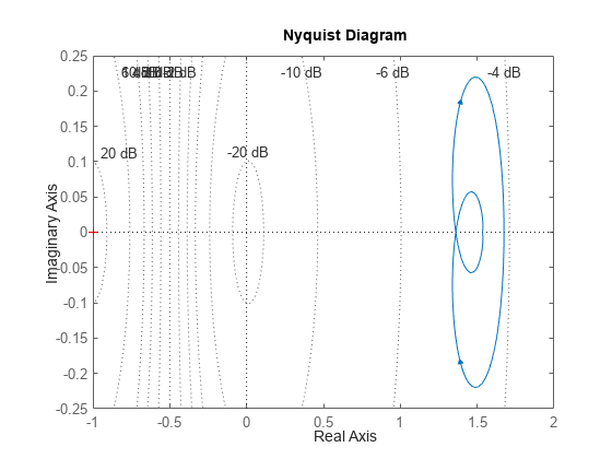
You can use the same option set to create multiple Nyquist plots with the same customization. Depending on your own toolbox preferences, the plot you obtain might look different from this plot. Only the properties that you set explicitly, in this example PhaseUnits and Grid, override the toolbox preferences.
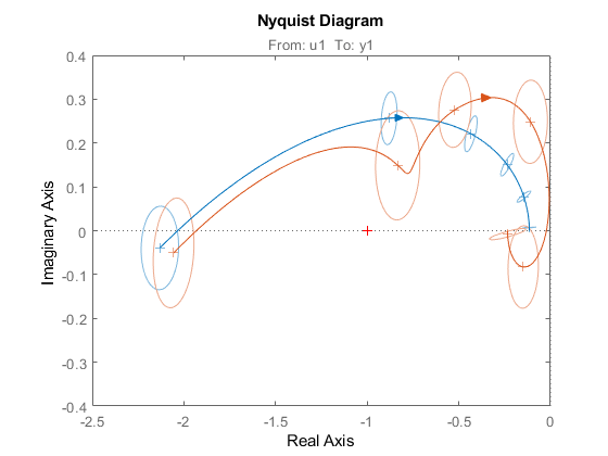
Compare the frequency responses of identified state-space models of order 2 and 6 along with their 1-std confidence regions rendered at every 50th frequency sample.

Load the identified model data and estimate the state-space models using n4sid. Then, plot the Nyquist diagram.

load iddata1
sys1 = n4sid(z1,2); 
sys2 = n4sid(z1,6);
w = linspace(10,10*pi,256);
h = nyquistplot(sys1,sys2,w);

Figure contains an axes object. The axes object with title From: u1 To: y1 contains 2 objects of type line. These objects represent sys1, sys2.

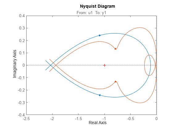
Both models produce about 76% fit to data. However, sys2 shows higher uncertainty in its frequency response, especially close to Nyquist frequency as shown by the plot. To see this, show the confidence region at a subset of the points at which the Nyquist response is displayed.

setoptions(h,'ConfidenceRegionDisplaySpacing',50,...
             'ShowFullContour','off');

Figure contains an axes object. The axes object with title From: u1 To: y1 contains 2 objects of type line. These objects represent sys1, sys2.

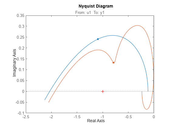
To turn on the confidence region display, right-click the plot and select Characteristics > Confidence Region.

nyquistplot_conf.png

For this example, consider a MIMO state-space model with 3 inputs, 3 outputs and 3 states. Create a Nyquist plot, display only the partial contour and turn the grid on.

Create the MIMO state-space model sys_mimo.

J = [8 -3 -3; -3 8 -3; -3 -3 8];
F = 0.2*eye(3);
A = -J\F;
B = inv(J);
C = eye(3);
D = 0;
sys_mimo = ss(A,B,C,D);
size(sys_mimo)
State-space model with 3 outputs, 3 inputs, and 3 states.

Create a Nyquist plot with plot handle h and use getoptions for a list of the options available.

h = nyquistplot(sys_mimo);
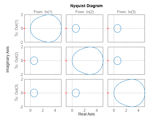
Figure contains 9 axes objects. Axes object 1 with title From: In(1), ylabel To: Out(1) contains an object of type line. This object represents sys\_mimo. Axes object 2 with ylabel To: Out(2) contains an object of type line. This object represents sys\_mimo. Axes object 3 with ylabel To: Out(3) contains an object of type line. This object represents sys\_mimo. Axes object 4 with title From: In(2) contains an object of type line. This object represents sys\_mimo. Axes object 5 contains an object of type line. This object represents sys\_mimo. Axes object 6 contains an object of type line. This object represents sys\_mimo. Axes object 7 with title From: In(3) contains an object of type line. This object represents sys\_mimo. Axes object 8 contains an object of type line. This object represents sys\_mimo. Axes object 9 contains an object of type line. This object represents sys\_mimo.

p = getoptions(h)
p =

                         FreqUnits: 'rad/s'
                          MagUnits: 'dB'
                        PhaseUnits: 'deg'
                   ShowFullContour: 'on'
          ConfidenceRegionNumberSD: 1
    ConfidenceRegionDisplaySpacing: 5
                        IOGrouping: 'none'
                       InputLabels: [1x1 struct]
                      OutputLabels: [1x1 struct]
                      InputVisible: {3x1 cell}
                     OutputVisible: {3x1 cell}
                             Title: [1x1 struct]
                            XLabel: [1x1 struct]
                            YLabel: [1x1 struct]
                         TickLabel: [1x1 struct]
                              Grid: 'off'
                         GridColor: [0.1500 0.1500 0.1500]
                              XLim: {3x1 cell}
                              YLim: {3x1 cell}
                          XLimMode: {3x1 cell}
                          YLimMode: {3x1 cell}

Use setoptions to update the plot with the requires customization.

setoptions(h,'ShowFullContour','off','Grid','on');

Figure contains 9 axes objects. Axes object 1 with title From: In(1), ylabel To: Out(1) contains an object of type line. This object represents sys\_mimo. Axes object 2 with ylabel To: Out(2) contains an object of type line. This object represents sys\_mimo. Axes object 3 with ylabel To: Out(3) contains an object of type line. This object represents sys\_mimo. Axes object 4 with title From: In(2) contains an object of type line. This object represents sys\_mimo. Axes object 5 contains an object of type line. This object represents sys\_mimo. Axes object 6 contains an object of type line. This object represents sys\_mimo. Axes object 7 with title From: In(3) contains an object of type line. This object represents sys\_mimo. Axes object 8 contains an object of type line. This object represents sys\_mimo. Axes object 9 contains an object of type line. This object represents sys\_mimo.

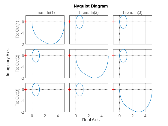
The Nyquist plot automatically updates when you call setoptions. For MIMO models, nyquistplot produces an array of Nyquist diagrams, each plot displaying the frequency response of one I/O pair.

Version History

Introduced in R2011a