Delay and Latency
Computational Delay
The computational delay of a block or subsystem is related to the number of operations involved in executing that block or subsystem. For example, an FFT block operating on a 256-sample input requires Simulink® software to perform a certain number of multiplications for each input frame. The actual amount of time that these operations consume depends heavily on the performance of both the computer hardware and underlying software layers, such as the MATLAB® environment and the operating system. Therefore, computational delay for a particular model can vary from one computer platform to another.
The simulation time represented on a model status bar, which can be accessed via the Simulink Digital Clock block, does not provide any information about computational delay. For example, according to the Simulink timer, the FFT mentioned above executes instantaneously, with no delay whatsoever. An input to the FFT block at simulation time t=25.0 is processed and output at simulation time t=25.0, regardless of the number of operations performed by the FFT algorithm. The Simulink timer reflects only algorithmic delay, not computational delay.
Reduce Computational Delay
There are a number of ways to reduce computational delay without actually running the simulation on faster hardware. To begin with, you should familiarize yourself with Manual Performance Optimization (Simulink) which describes some basic strategies. The following information discusses several options for improving performance.
A first step in improving performance is to analyze your model, and eliminate or simplify elements that are adding excessively to the computational load. Such elements might include scope displays and data logging blocks that you had put in place for debugging purposes and no longer require. In addition to these model-specific adjustments, there are a number of more general steps you can take to improve the performance of any model:
Use frame-based processing wherever possible. It is advantageous for the entire model to be frame based. See Benefits of Frame-Based Processing for more information.
Use the DSP Simulink model templates to tailor Simulink for digital signal processing modeling. For more information, see Configure the Simulink Environment for Signal Processing Models.
Turn off the Simulink status bar. In the Modeling tab, deselect Environment > Status Bar. Simulation speed will improve, but the time indicator will not be visible.
Run your simulation from the MATLAB command line by typing
sim(gcs)
This method of starting a simulation can greatly increase the simulation speed, but also has several limitations:
You cannot interact with the simulation (to tune parameters, for instance).
You must press Ctrl+C to stop the simulation, or specify start and stop times.
There are no graphics updates in MATLAB S-functions.
Use Simulink Coder™ code generation software to generate generic real-time (GRT) code targeted to your host platform, and run the model using the generated executable file. See the Simulink Coder documentation for more information.
Algorithmic Delay
Algorithmic delay is delay that is intrinsic to the algorithm of a block or subsystem and is independent of CPU speed. In this guide, the algorithmic delay of a block is referred to simply as the block delay. It is generally expressed in terms of the number of samples by which a block output lags behind the corresponding input. This delay is directly related to the time elapsed on the Simulink timer during the execution of the block.
The algorithmic delay of a particular block may depend on both the block parameter settings and the general Simulink settings. To simplify matters, it is helpful to categorize block delay using the following categories:
The following topics explain the different categories of delay, and how the simulation and parameter settings can affect the level of delay that a particular block experiences.
Zero Algorithmic Delay
The FFT block is an example of a component that has no algorithmic delay. The Simulink timer does not record any passage of time while the block computes the FFT of the input, and the transformed data is available at the output in the same time step that the input is received. There are many other blocks that have zero algorithmic delay, such as the blocks in the Matrices and Linear Algebra libraries. Each of those blocks processes its input and generates its output in a single time step.
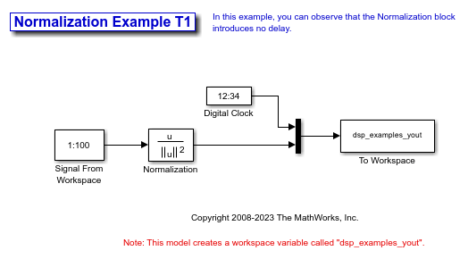
The Normalization block is an example of a block with zero algorithmic delay:
Open the ex_normalization_tut model.
Double-click the Signal From Workspace block. The Signal From Workspace dialog box opens.
Set the block parameters as follows:
Signal = 1:100
Sample time = 1/4
Samples per frame = 4
Save these parameters and close the dialog box by clicking OK.
Run the model.
The model prepends the current value of the Simulink timer output from the Digital Clock block to each output frame.
The Signal From Workspace block generates a new frame containing four samples once every second (Tfo = 4*  ). The first few output frames are:
(t = 0): [ 1 2 3 4]'
(t = 1): [ 5 6 7 8]'
(t = 2): [ 9 10 11 12]'
(t = 3): [13 14 15 16]'
(t = 4): [17 18 19 20]'
At the MATLAB command prompt, type squeeze(dsp_examples_yout)'.
The normalized output dsp_examples_yout is converted to an easier-to-read matrix format.
The first column of the output is the Simulink time provided by the Digital Clock block. You can see that the squared 2-norm of the first input, [1 2 3 4]' ./ sum([1 2 3 4]'.^2) appears in the first row of the output (at time t = 0), the same time step that the input was received by the block. This indicates that the Normalization block has zero algorithmic delay.
Zero Algorithmic Delay and Algebraic Loops
When several blocks with zero algorithmic delay are connected in a feedback loop, Simulink may report an algebraic loop error and performance may generally suffer. You can prevent algebraic loops by injecting at least one sample of delay into a feedback loop, for example, by including a Delay block with Delay greater than 0. For more information, see Algebraic Loop Concepts (Simulink).
Basic Algorithmic Delay
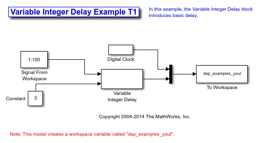
The Variable Integer Delay block is an example of a block with algorithmic delay. In the following example, you use this block to demonstrate this concept:
Open the ex_variableintegerdelay_tut model.
Double-click the Signal From Workspace block. The Signal From Workspace dialog box opens.
Set the block parameters as follows:
Signal = 1:100
Sample time = 1
Samples per frame = 1
Save these parameters and close the dialog box by clicking OK.
Double-click the Constant block. The Constant dialog box opens.
Set the block parameters as follows:
Constant value = 3
Clear the Interpret vector parameters as 1-D parameter
Sample time = 1
Click OK to save these parameters and close the dialog box.
The input to the Delay port of the Variable Integer Delay block specifies the number of sample periods that should elapse before an input to the In port is released to the output. This value represents the algorithmic delay of the block.
In this example, since the input to the Delay port is 3 and the sample period at the In and Delay ports is 1 then the sample that arrives at the In port of the block at time t = 0 is released to the output at time t = 3.
Double-click the Variable Integer Delay block. The Variable Integer Delay dialog box opens.
Set the Initial conditions parameter to -1, and then click OK.
In the Debug tab, under Information Overlays, select Signal Dimensions and Nonscalar Signals.
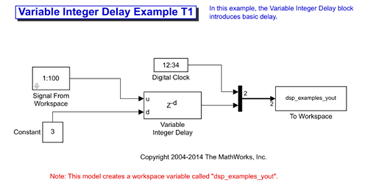
Run the model. The model should look similar to the following figure.
At the MATLAB® command prompt, type dsp_examples_yout. The output is shown below:
dsp_examples_yout =

     0    -1
     1    -1
     2    -1
     3     1
     4     2
     5     3
The first column is the Simulink time provided by the Digital Clock block. The second column is the delayed input. As expected, the input to the block at t = 0 is delayed three samples and appears as the fourth output sample, at t = 3. You can also see that the first three outputs from the Variable Integer Delay block inherit the value of the block Initial conditions parameter, -1. This period of time, from the start of the simulation until the first input is propagated to the output, is sometimes called the initial delay of the block.
Many DSP System Toolbox blocks have some degree of fixed or adjustable algorithmic delay. These include any blocks whose algorithms rely on delay or storage elements, such as filters or buffers. Often, but not always, such blocks provide an Initial conditions parameter that allows you to specify the output values generated by the block during the initial delay. In other cases, the initial conditions are internally set to 0.
Consult the block reference pages for the delay characteristics of specific DSP System Toolbox blocks.
Excess Algorithmic Delay (Tasking Latency)
Under certain conditions, Simulink may force a block to delay inputs longer than is strictly required by the block algorithm. This excess algorithmic delay is called tasking latency, because it arises from synchronization requirements of the Simulink tasking mode. The overall algorithmic delay of a block is the sum of its basic delay and tasking latency.
Algorithmic delay = Basic algorithmic delay + Tasking latency
The tasking latency for a particular block may be dependent on the following block and model characteristics:
Simulink Tasking Mode
Simulink has two tasking modes:
Single-tasking
Multitasking
In the Modeling tab, click Model
Settings. In the Solver pane,
select Type > Fixed-step.
Expand Solver details. To specify multitasking mode,
select Treat each discrete rate as a separate task. To
specify single-tasking mode, clear Treat each discrete rate as a
separate task.
Note
Many multirate blocks have reduced latency in the Simulink single-tasking mode. Check the “Latency” section of a multirate block reference page for details. Also see Time-Based Scheduling and Code Generation (Simulink Coder).
Block Rate Type
A block is called single-rate when all of its input and output ports operate at the same frame rate. A block is called multirate when at least one input or output port has a different frame rate than the others.
Many blocks are permanently single-rate. This means that all input and output ports always have the same frame rate. For other blocks, the block parameter settings determine whether the block is single-rate or multirate. Only multirate blocks are subject to tasking latency.
Note
Simulink may report an algebraic loop error if it detects a feedback loop composed entirely of multirate blocks. To break such an algebraic loop, insert a single-rate block with nonzero delay, such as a Unit Delay block. For more information, see Algebraic Loop Concepts (Simulink).
Model Rate Type
When all ports of all blocks in a model operate at a single frame rate, the model is called single-rate. When the model contains blocks with differing frame rates, or at least one multirate block, the model is called multirate. Note that Simulink prevents a single-rate model from running in multitasking mode by generating an error.
Block Input Processing Mode
Many blocks can operate in either sample-based or frame-based processing
modes. To choose, you can set the Input processing
parameter of the block to Columns as channels (frame
based) or Elements as channels (sample
based).
Predict Tasking Latency
The specific amount of tasking latency created by a particular combination of block parameter and simulation settings is discussed in the 'Latency' section of a block reference page. In this topic, you use the Upsample block reference page to predict the tasking latency of a model:
Open the ex_upsample_tut1 model. The Upsample Example T1 model opens.
In the Modeling tab, click Model Settings.
In the Solver pane, from the Type list, select Fixed-step. From the Solver list, select discrete (no continuous states).
Expand Solver details. Select Treat each discrete rate as a separate task and click OK. Most multirate blocks experience tasking latency only in the Simulink multitasking mode.
Double-click the Signal From Workspace block. The Signal From Workspace dialog box opens.
Set the block parameters as follows, and then click OK:
Signal = 1:100
Sample time = 1/4
Samples per frame = 4
Form output after final data value by =
Setting to zero
Double-click the Upsample block. The Upsample dialog box opens.
Set the block parameters as follows, and then click OK:
Upsample factor, L = 4
Sample offset (0 to L-1) = 0
Input processing =
Columns as channels (frame based)Rate options =
Allow multirate processingInitial conditions = -1
The Rate options parameter makes the model multirate, since the input and output frame rates will not be equal.
Double-click the Digital Clock block. The Digital Clock dialog box opens.
Set Sample time to 0.25, and then click OK. This matches the sample period of the Upsample block output.
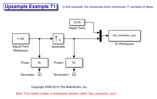
Run the model. The model should now look similar to the following figure.
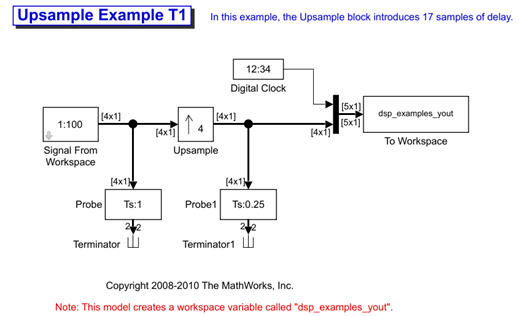
The model prepends the current value of the Simulink timer, from the Digital Clock block, to each output frame.
In the example, the Signal From Workspace block generates a new frame containing four samples once every second ( ). The first few output frames are:
(t = 0): [ 1 2 3 4]
(t = 1): [ 5 6 7 8]
(t = 2): [ 9 10 11 12]
(t = 3): [13 14 15 16]
(t = 4): [17 18 19 20]
The Upsample block upsamples the input by a factor of 4, inserting three zeros between each input sample. The change in rates is confirmed by the Probe blocks in the model, which show a decrease in the frame period from  to
to  .
.
At the MATLAB command prompt, type squeeze(dsp_examples_yout)'.
The output from the simulation is displayed in a matrix format. The first few samples of the result, ans, are:
'Latency and Initial Conditions' in the Upsample block reference page indicates that when Simulink is in multitasking mode, the first sample of the block input appears in the output as sample  , where Mi is the input frame size, L is the Upsample factor, L, and D is the Sample offset. This formula predicts that the first input in this example should appear as output sample 17 (that is, 4*4+0+1).
The first column of the output is the Simulink time provided by the Digital Clock block. The four values to the right of each time are the values in the output frame at that time. You can see that the first sample in each of the first four output frames inherits the value of the Upsample block Initial conditions parameter. As a result of the tasking latency, the first input value appears as the first sample of the 5th output frame at t = 1. This is sample 17.
Now try running the model in single-tasking mode.
In the Modeling tab, click Model Settings.
In the Solver pane, from the Type list, select Fixed-step. From the Solver list, select Discrete (no continuous states).
Clear the Treat each discrete rate as a separate task parameter.
Run the model. The model now runs in single-tasking mode.
At the MATLAB command prompt, type squeeze(dsp_examples_yout)'. The first few samples of the result, ans, are:
'Latency and Initial Conditions' in the Upsample block reference page indicates that the block has zero latency for all multirate operations in the Simulink single-tasking mode.
The first column of the output is the Simulink time provided by the Digital Clock block. The four values to the right of each time are the values in the output frame at that time. The first input value appears as the first sample of the first output frame (at t = 0). This is the expected behavior for the zero-latency condition. For the particular parameter settings used in this example, running upsample_tut1 in single-tasking mode eliminates the 17-sample delay that is present when you run the model in multitasking mode.
You have now successfully used the Upsample block reference page to predict the tasking latency of a model.
Related Topics
You can also select a web site from the following list:
Americas
- América Latina (Español)
- Canada (English)
- United States (English)
Europe
- Belgium (English)
- Denmark (English)
- Deutschland (Deutsch)
- España (Español)
- Finland (English)
- France (Français)
- Ireland (English)
- Italia (Italiano)
- Luxembourg (English)
- Netherlands (English)
- Norway (English)
- Österreich (Deutsch)
- Portugal (English)
- Sweden (English)
- Switzerland
- United Kingdom (English)