ilu
Incomplete LU factorization
Description
[___] = ilu(
performs the incomplete LU factorization of A,options)A with options specified
by the structure options.
For example, you can perform an incomplete LU factorization with pivoting by setting
the type field of options to
"ilutp". You can then specify a row-sum or column-sum preserving
modified incomplete LU factorization by setting the milu field to
"row" or "col". This combination of options
returns the permutation matrix P such that L and
U are incomplete factors of A*P for the
"row" option (where U is column permuted), or
L and U are incomplete factors of
P*A for the "col" option (where
L is row permuted).
Examples
Different Types of Incomplete LU Factorization
The ilu function provides three types of incomplete LU factorizations: the zero-fill factorization (ILU(0)), the Crout version (ILUC), and the factorization with threshold dropping and pivoting (ILUTP).
By default, ilu performs the zero-fill incomplete LU factorization of a sparse matrix input. For example, find the complete and incomplete factorization of a sparse matrix with 7840 nonzeros. Its complete LU factors have 126,478 nonzeros, and its incomplete LU factors with zero-fill have 7840 nonzeros, the same number as A.
A = gallery("neumann",1600) + speye(1600);
n = nnz(A)
n = 7840
n = nnz(lu(A))
n = 126478
n = nnz(ilu(A))
n = 7840
Because the zero-fill factorization preserves the sparsity pattern of the input matrix in its LU factors, the relative error of the factorization is essentially zero on the pattern of nonzero elements of A.
[L,U] = ilu(A);
e = norm(A-(L*U).*spones(A),"fro")/norm(A,"fro")
e = 4.8874e-17
However, the product of these zero-fill factors is not a good approximation of the original matrix.
e = norm(A-L*U,"fro")/norm(A,"fro")
e = 0.0601
To improve the accuracy, you can use other types of incomplete LU factorization with fill-in. For example, use the Crout version with a 1e-6 drop tolerance.
options.droptol = 1e-6;
options.type = "crout";
[L,U] = ilu(A,options);
The Crout version of the incomplete factorization has 51,482 nonzeros in its LU factors (less than the complete factorization). With fill-in, the product of the incomplete LU factors is a better approximation of the original matrix.
n = nnz(ilu(A,options))
n = 51482
e = norm(A-L*U,"fro")./norm(A,"fro")
e = 9.3040e-07
For comparison, for the same input matrix A, the incomplete factorization with threshold dropping and pivoting gives results similar to the Crout version.
options.type = "ilutp";
[L,U,P] = ilu(A,options);
n = nnz(ilu(A,options))
n = 51541
norm(P*A-L*U,"fro")./norm(A,"fro")
ans = 9.4960e-07
Drop Tolerance of Incomplete LU Factorization
Change the drop tolerance of incomplete LU factorization to factor a sparse matrix.
Load the west0479 matrix, which is a real-valued 479-by-479 nonsymmetric sparse matrix. Estimate the condition number of the matrix by using condest.
load west0479
A = west0479;
c1 = condest(A)
c1 = 1.4244e+12
Improve the condition number of the matrix by using equilibrate. Permute and rescale the original matrix A to create a new matrix B = R*P*A*C, which has a better condition number and diagonal entries of only 1 and –1.
[P,R,C] = equilibrate(A);
B = R*P*A*C;
c2 = condest(B)
c2 = 5.1036e+04
Specify the options to perform the incomplete LU factorization of B with threshold dropping and pivoting that preserves the row sum. For comparison purposes, first specify a zero drop tolerance of fill-in, which produces the complete LU factorization.
options.type = "ilutp";
options.milu = "row";
options.droptol = 0;
[L,U,P] = ilu(B,options);
This factorization is very accurate in approximating the input matrix B, but the factors are significantly more dense than B.
e = norm(B*P-L*U,"fro")/norm(B,"fro")
e = 1.0345e-16
nLU = nnz(L)+nnz(U)-size(B,1)
nLU = 19118
nB = nnz(B)
nB = 1887
You can change the drop tolerance to obtain incomplete LU factors that are more sparse but less accurate in approximating B. For example, the following plots show the ratio of the density of the incomplete factors to the density of the input matrix plotted against the drop tolerance, and the relative error of the incomplete factorization.
ntols = 20;
tau = logspace(-6,-2,ntols);
e = zeros(1,ntols);
nLU = zeros(1,ntols);
for k = 1:ntols
    options.droptol = tau(k);
    [L,U,P] = ilu(B,options);
    nLU(k) = nnz(L)+nnz(U)-size(B,1);
    e(k) = norm(B*P-L*U,"fro")/norm(B,"fro");
end
figure
semilogx(tau,nLU./nB,LineWidth=2)
title("Ratio of nonzeros of LU factors with respect to B")
xlabel("drop tolerance")
ylabel("nnz(L)+nnz(U)-size(B,1)/nnz(B)",FontName="FixedWidth")
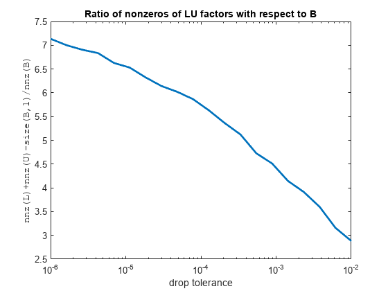
figure
loglog(tau,e,LineWidth=2)
title("Relative error of the incomplete LU factorization")
xlabel("drop tolerance")
ylabel("$||BP-LU||_F\,/\,||B||_F$",Interpreter="latex")
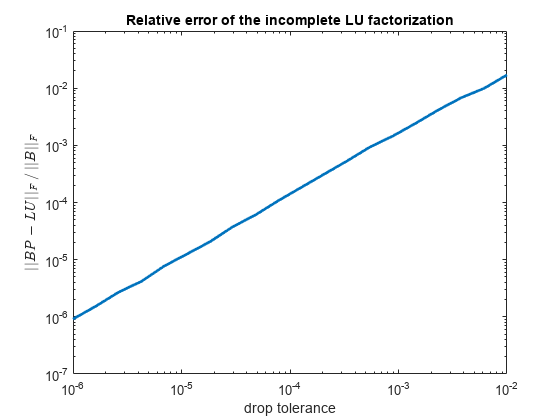
In this example, the relative error of the incomplete LU factorization with threshold dropping is on the same order of the drop tolerance (which does not always occur).
Using ilu as Preconditioner to Solve Linear System
Use an incomplete LU factorization as a preconditioner for bicgstab to solve a linear system.
Load west0479, a real 479-by-479 nonsymmetric sparse matrix.
load west0479
A = west0479;
Define b so that the true solution to is a vector of all ones.
b = full(sum(A,2));
Set the tolerance and maximum number of iterations.
tol = 1e-12;
maxit = 20;
Use bicgstab to find a solution at the requested tolerance and number of iterations. Specify five outputs to return information about the solution process:
xis the computed solution toA*x = b.fl0is a flag indicating whether the algorithm converged.rr0is the relative residual of the computed answerx.it0is the iteration number whenxwas computed.rv0is a vector of the residual history at each half iteration for .
[x,fl0,rr0,it0,rv0] = bicgstab(A,b,tol,maxit);
fl0
fl0 = 1
rr0
rr0 = 1
it0
it0 = 0
fl0 is 1 because bicgstab does not converge to the requested tolerance 1e-12 within the requested 20 iterations. In fact, the behavior of bicgstab is so poor that the initial guess x0 = zeros(size(A,2),1) is the best solution and is returned, as indicated by it0 = 0.
To aid with the slow convergence, you can specify a preconditioner matrix. Because A is nonsymmetric, use ilu to generate the preconditioner . Specify a drop tolerance to ignore nondiagonal entries with values smaller than 1e-6. Solve the preconditioned system by specifying L and U as inputs to bicgstab.
options = struct("type","ilutp","droptol",1e-6);
[L,U] = ilu(A,options);
[x_precond,fl1,rr1,it1,rv1] = bicgstab(A,b,tol,maxit,L,U);
fl1
fl1 = 0
rr1
rr1 = 5.9892e-14
it1
it1 = 3
The use of an ilu preconditioner produces a relative residual rr1 less than the requested tolerance of 1e-12 at the third iteration. The output rv1(1) is norm(b), and the output rv1(end) is norm(b-A*x1).
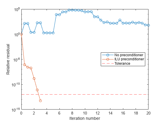
You can follow the progress of bicgstab by plotting the relative residuals at each half iteration. Plot the residual history of each solution with a line for the specified tolerance.
semilogy((0:numel(rv0)-1)/2,rv0/norm(b),"-o")
hold on
semilogy((0:numel(rv1)-1)/2,rv1/norm(b),"-o")
yline(tol,"r--");
legend("No preconditioner","ILU preconditioner","Tolerance",Location="East")
xlabel("Iteration number")
ylabel("Relative residual")
Input Arguments
Output Arguments
Tips
The incomplete factorizations returned by this function may be useful as preconditioners for a system of linear equations being solved by iterative methods, such as
bicg,bicgstab, orgmres.
References
[1] Saad, Y. "Preconditioning Techniques", chap. 10 in Iterative Methods for Sparse Linear Systems. The PWS Series in Computer Science. Boston: PWS Pub. Co, 1996.
Extended Capabilities
Version History
Introduced in R2007a
See Also
You can also select a web site from the following list:
Americas
- América Latina (Español)
- Canada (English)
- United States (English)
Europe
- Belgium (English)
- Denmark (English)
- Deutschland (Deutsch)
- España (Español)
- Finland (English)
- France (Français)
- Ireland (English)
- Italia (Italiano)
- Luxembourg (English)
- Netherlands (English)
- Norway (English)
- Österreich (Deutsch)
- Portugal (English)
- Sweden (English)
- Switzerland
- United Kingdom (English)