mkpp
Make piecewise polynomial
Description
Examples
Create Piecewise Polynomial with Polynomials of Several Degrees
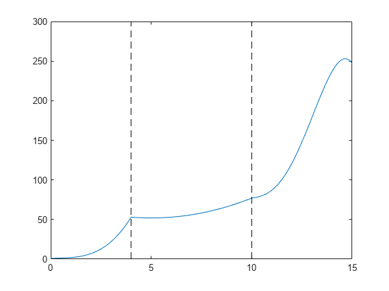
Create a piecewise polynomial that has a cubic polynomial in the interval [0,4], a quadratic polynomial in the interval [4,10], and a quartic polynomial in the interval [10,15].
breaks = [0 4 10 15];
coefs = [0 1 -1 1 1; 0 0 1 -2 53; -1 6 1 4 77];
pp = mkpp(breaks,coefs)
pp = struct with fields:
      form: 'pp'
    breaks: [0 4 10 15]
     coefs: [3x5 double]
    pieces: 3
     order: 5
       dim: 1
Evaluate the piecewise polynomial at many points in the interval [0,15] and plot the results. Plot vertical dashed lines at the break points where the polynomials meet.
xq = 0:0.01:15;
plot(xq,ppval(pp,xq))
line([4 4],ylim,'LineStyle','--','Color','k')
line([10 10],ylim,'LineStyle','--','Color','k')
Create Piecewise Polynomial with Repeated Pieces
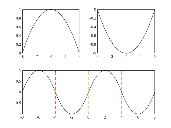
Create and plot a piecewise polynomial with four intervals that alternate between two quadratic polynomials.
The first two subplots show a quadratic polynomial and its negation shifted to the intervals [-8,-4] and [-4,0]. The polynomial is
The third subplot shows a piecewise polynomial constructed by alternating these two quadratic pieces over four intervals. Vertical lines are added to show the points where the polynomials meet.
subplot(2,2,1)
cc = [-1/4 1 0];
pp1 = mkpp([-8 -4],cc);
xx1 = -8:0.1:-4;
plot(xx1,ppval(pp1,xx1),'k-')

subplot(2,2,2)
pp2 = mkpp([-4 0],-cc);
xx2 = -4:0.1:0;
plot(xx2,ppval(pp2,xx2),'k-')

subplot(2,1,2)
pp = mkpp([-8 -4 0 4 8],[cc;-cc;cc;-cc]);
xx = -8:0.1:8;
plot(xx,ppval(pp,xx),'k-')
hold on
line([-4 -4],ylim,'LineStyle','--')
line([0 0],ylim,'LineStyle','--')
line([4 4],ylim,'LineStyle','--')
hold off
Input Arguments
Output Arguments
Extended Capabilities
Version History
Introduced before R2006a
You can also select a web site from the following list:
Americas
- América Latina (Español)
- Canada (English)
- United States (English)
Europe
- Belgium (English)
- Denmark (English)
- Deutschland (Deutsch)
- España (Español)
- Finland (English)
- France (Français)
- Ireland (English)
- Italia (Italiano)
- Luxembourg (English)
- Netherlands (English)
- Norway (English)
- Österreich (Deutsch)
- Portugal (English)
- Sweden (English)
- Switzerland
- United Kingdom (English)