pcg
Solve system of linear equations — preconditioned conjugate gradients method
Syntax
Description
x = pcg(A,b)A*x = b for
x using the Preconditioned Conjugate Gradients Method. When the attempt is
successful, pcg displays a message to confirm convergence. If
pcg fails to converge after the maximum number of iterations or halts
for any reason, it displays a diagnostic message that includes the relative residual
norm(b-A*x)/norm(b) and the iteration number at which the method
stopped.
[
returns a flag that specifies whether the algorithm successfully converged. When
x,flag] = pcg(___)flag = 0, convergence was successful. You can use this output syntax
with any of the previous input argument combinations. When you specify the
flag output, pcg does not display any diagnostic
messages.
Examples
Iterative Solution to Linear System
Solve a square linear system using pcg with default settings, and then adjust the tolerance and number of iterations used in the solution process.
Create a random symmetric sparse matrix A. Also create a vector b of the row sums of A for the right-hand side of so that the true solution is a vector of ones.
rng default
A = sprand(400,400,.5);
A = A'*A;
b = sum(A,2);
Solve using pcg. The output display includes the value of the relative residual error .
x = pcg(A,b);
pcg stopped at iteration 20 without converging to the desired tolerance 1e-06
because the maximum number of iterations was reached.
The iterate returned (number 20) has relative residual 3.6e-06.
By default pcg uses 20 iterations and a tolerance of 1e-6, and the algorithm is unable to converge in those 20 iterations for this matrix. However, the residual is close to the tolerance, so the algorithm likely just needs more iterations to converge.
Solve the system again using a tolerance of 1e-7 and 150 iterations.
x = pcg(A,b,1e-7,150);
pcg converged at iteration 129 to a solution with relative residual 1e-07.
Using pcg with Preconditioner
Examine the effect of using a preconditioner matrix with pcg to solve a linear system.
Create a symmetric positive definite, banded coefficient matrix.
A = delsq(numgrid('S',102));Define b for the right-hand side of the linear equation .
b = ones(size(A,1),1);
Set the tolerance and maximum number of iterations.
tol = 1e-8;
maxit = 100;
Use pcg to find a solution at the requested tolerance and number of iterations. Specify five outputs to return information about the solution process:
xis the computed solution toA*x = b.fl0is a flag indicating whether the algorithm converged.rr0is the relative residual of the computed answerx.it0is the iteration number whenxwas computed.rv0is a vector of the residual history for .
[x,fl0,rr0,it0,rv0] = pcg(A,b,tol,maxit);
fl0
fl0 = 1
rr0
rr0 = 0.0131
it0
it0 = 100
fl0 is 1 because pcg does not converge to the requested tolerance of 1e-8 within the requested 100 iterations.
To aid with the slow convergence, you can specify a preconditioner matrix. Since A is symmetric, use ichol to generate the preconditioner . Solve the preconditioned system by specifying L and L' as inputs to pcg.
L = ichol(A);
[x1,fl1,rr1,it1,rv1] = pcg(A,b,tol,maxit,L,L');
fl1
fl1 = 0
rr1
rr1 = 8.0992e-09
it1
it1 = 79
The use of an ichol preconditioner produces a relative residual less than the prescribed tolerance of 1e-8 at the 79th iteration. The output rv1(1) is norm(b) and rv1(end) is norm(b-A*x1).
Now, use the michol option to create a modified incomplete Cholesky preconditioner.
L = ichol(A,struct('michol','on'));
[x2,fl2,rr2,it2,rv2] = pcg(A,b,tol,maxit,L,L');
fl2
fl2 = 0
rr2
rr2 = 9.9614e-09
it2
it2 = 47
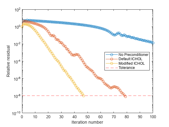
This preconditioner is better than the one produced by the incomplete Cholesky factorization with zero fill for the coefficient matrix in this example, so pcg is able to converge even quicker.
You can see how the preconditioners affect the rate of convergence of pcg by plotting each of the residual histories starting from the initial estimate (iterate number 0). Add a line for the specified tolerance.
semilogy(0:length(rv0)-1,rv0/norm(b),'-o')
hold on
semilogy(0:length(rv1)-1,rv1/norm(b),'-o')
semilogy(0:length(rv2)-1,rv2/norm(b),'-o')
yline(tol,'r--');
legend('No Preconditioner','Default ICHOL','Modified ICHOL','Tolerance','Location','East')
xlabel('Iteration number')
ylabel('Relative residual')
Supplying Initial Guess
Examine the effect of supplying pcg with an initial guess of the solution.
Create a tridiagonal sparse matrix. Use the sum of each row as the vector for the right-hand side of so that the expected solution for is a vector of ones.
n = 900;
e = ones(n,1);
A = spdiags([e 2*e e],-1:1,n,n);
b = sum(A,2);
Use pcg to solve twice: one time with the default initial guess, and one time with a good initial guess of the solution. Use 200 iterations and the default tolerance for both solutions. Specify the initial guess in the second solution as a vector with all elements equal to 0.99.
maxit = 200;
x1 = pcg(A,b,[],maxit);
pcg converged at iteration 35 to a solution with relative residual 9.5e-07.
x0 = 0.99*e;
x2 = pcg(A,b,[],maxit,[],[],x0);
pcg converged at iteration 7 to a solution with relative residual 8.7e-07.
In this case supplying an initial guess enables pcg to converge more quickly.
Returning Intermediate Results
You also can use the initial guess to get intermediate results by calling pcg in a for-loop. Each call to the solver performs a few iterations and stores the calculated solution. Then you use that solution as the initial vector for the next batch of iterations.
For example, this code performs 100 iterations four times and stores the solution vector after each pass in the for-loop:
x0 = zeros(size(A,2),1);
tol = 1e-8;
maxit = 100;
for k = 1:4
    [x,flag,relres] = pcg(A,b,tol,maxit,[],[],x0);
    X(:,k) = x;
    R(k) = relres;
    x0 = x;
end
X(:,k) is the solution vector computed at iteration k of the for-loop, and R(k) is the relative residual of that solution.
Using Function Handle Instead of Numeric Matrix
Solve a linear system by providing pcg with a function handle that computes A*x in place of the coefficient matrix A.
Use gallery to generate a 20-by-20 positive definite tridiagonal matrix. The super- and subdiagonals have ones, while the main diagonal elements count down from 20 to 1. Preview the matrix.
n = 20;
A = gallery('tridiag',ones(n-1,1),n:-1:1,ones(n-1,1));
full(A)
ans = 20×20
20 1 0 0 0 0 0 0 0 0 0 0 0 0 0 0 0 0 0 0
1 19 1 0 0 0 0 0 0 0 0 0 0 0 0 0 0 0 0 0
0 1 18 1 0 0 0 0 0 0 0 0 0 0 0 0 0 0 0 0
0 0 1 17 1 0 0 0 0 0 0 0 0 0 0 0 0 0 0 0
0 0 0 1 16 1 0 0 0 0 0 0 0 0 0 0 0 0 0 0
0 0 0 0 1 15 1 0 0 0 0 0 0 0 0 0 0 0 0 0
0 0 0 0 0 1 14 1 0 0 0 0 0 0 0 0 0 0 0 0
0 0 0 0 0 0 1 13 1 0 0 0 0 0 0 0 0 0 0 0
0 0 0 0 0 0 0 1 12 1 0 0 0 0 0 0 0 0 0 0
0 0 0 0 0 0 0 0 1 11 1 0 0 0 0 0 0 0 0 0
⋮
Since this tridiagonal matrix has a special structure, you can represent the operation A*x with a function handle. When A multiplies a vector, most of the elements in the resulting vector are zeros. The nonzero elements in the result correspond with the nonzero tridiagonal elements of A. Moreover, only the main diagonal has nonzeros that are not equal to 1.
The expression becomes:
.
The resulting vector can be written as the sum of three vectors:
=.
In MATLAB®, write a function that creates these vectors and adds them together, thus giving the value of A*x:
function y = afun(x)
y = [0; x(1:19)] + ...
    [(20:-1:1)'].*x + ...
    [x(2:20); 0];
end
(This function is saved as a local function at the end of the example.)
Now, solve the linear system by providing pcg with the function handle that calculates A*x. Use a tolerance of 1e-12 and 50 iterations.
b = ones(20,1);
tol = 1e-12;
maxit = 50;
x1 = pcg(@afun,b,tol,maxit)
pcg converged at iteration 20 to a solution with relative residual 4.4e-16.
x1 = 20×1

    0.0476
    0.0475
    0.0500
    0.0526
    0.0555
    0.0588
    0.0625
    0.0666
    0.0714
    0.0769
      ⋮
Check that afun(x1) produces a vector of ones.
afun(x1)
ans = 20×1

    1.0000
    1.0000
    1.0000
    1.0000
    1.0000
    1.0000
    1.0000
    1.0000
    1.0000
    1.0000
      ⋮
Local Functions
function y = afun(x)
y = [0; x(1:19)] + ...
    [(20:-1:1)'].*x + ...
    [x(2:20); 0];
end
Input Arguments
Output Arguments
More About
Tips
Convergence of most iterative methods depends on the condition number of the coefficient matrix,
cond(A). WhenAis square, you can useequilibrateto improve its condition number, and on its own this makes it easier for most iterative solvers to converge. However, usingequilibratealso leads to better quality preconditioner matrices when you subsequently factor the equilibrated matrixB = R*P*A*C.You can use matrix reordering functions such as
dissectandsymrcmto permute the rows and columns of the coefficient matrix and minimize the number of nonzeros when the coefficient matrix is factored to generate a preconditioner. This can reduce the memory and time required to subsequently solve the preconditioned linear system.
References
[1] Barrett, R., M. Berry, T. F. Chan, et al., Templates for the Solution of Linear Systems: Building Blocks for Iterative Methods, SIAM, Philadelphia, 1994.
Extended Capabilities
Version History
Introduced before R2006a
You can also select a web site from the following list:
Americas
- América Latina (Español)
- Canada (English)
- United States (English)
Europe
- Belgium (English)
- Denmark (English)
- Deutschland (Deutsch)
- España (Español)
- Finland (English)
- France (Français)
- Ireland (English)
- Italia (Italiano)
- Luxembourg (English)
- Netherlands (English)
- Norway (English)
- Österreich (Deutsch)
- Portugal (English)
- Sweden (English)
- Switzerland
- United Kingdom (English)