pdepe
Solve 1-D parabolic and elliptic PDEs
Syntax
Description
sol = pdepe(m,pdefun,icfun,bcfun,xmesh,tspan)m represents the symmetry of the problem (slab,
cylindrical, or spherical). The equations being solved are coded in
pdefun, the initial value is coded in icfun, and the
boundary conditions are coded in bcfun. The ordinary differential
equations (ODEs) resulting from discretization in space are integrated to obtain approximate
solutions at the times specified in tspan. The pdepe
function returns values of the solution on a mesh provided in
xmesh.
[
also finds where functions of (t,u(x,t)), called event functions, are zero. In the output, sol,tsol,sole,te,ie] = pdepe(m,pdefun,icfun,bcfun,xmesh,tspan,options)te is
the time of the event, sole is the solution at the time of the event, and
ie is the index of the triggered event. tsol is a
column vector of times specified in tspan, prior to the first terminal
event.
For each event function, specify whether the integration is to terminate at a zero and
whether the direction of the zero-crossing matters. Do this by setting the
'Events' option of odeset to a function, such as
@myEventFcn, and creating a corresponding function:
[value,isterminal,direction] =
myEventFcn(m,t,xmesh,umesh).
The xmesh input contains the spatial mesh and umesh is
the solution at the mesh points.
Examples
Solve Heat Equation in Cylindrical Coordinates
Solve the heat equation in cylindrical coordinates using pdepe, and plot the solution.
In cylindrical coordinates with angular symmetry the heat equation is
The equation is defined for at times . The initial condition is defined in terms of the bessel function and its first zero as
Since this problem is in cylindrical coordinates (m = 1), pdepe automatically enforces the symmetry condition at . The right boundary condition is
The initial and boundary conditions are selected to be consistent with the analytic solution to the problem,
To solve this equation in MATLAB®, you need to code the equation, initial conditions, and boundary conditions, then select a suitable solution mesh before calling the solver pdepe. You either can include the required functions as local functions at the end of a file (as done here), or save them as separate, named files in a directory on the MATLAB path.
Code Equation
Before you can code the equation, you need to rewrite it in a form that the pdepe solver expects. The standard form that pdepe expects is
Written in this form, the PDE becomes
With the equation in the proper form you can read off the relevant terms:
Now you can create a function to code the equation. The function should have the signature [c,f,s] = heatcyl(x,t,u,dudx):
xis the independent spatial variable.tis the independent time variable.uis the dependent variable being differentiated with respect toxandt.dudxis the partial spatial derivative .The outputs
c,f, andscorrespond to coefficients in the standard PDE equation form expected bypdepe. These coefficients are coded in terms of the input variablesx,t,u, anddudx.
As a result, the equation in this example can be represented by the function:
function [c,f,s] = heatcyl(x,t,u,dudx)
c = 1;
f = dudx;
s = 0;
end
(Note: All functions are included as local functions at the end of the example.)
Code Initial Conditions
Next, write a function that returns the initial condition. The initial condition is applied at the first time value tspan(1). The function should have the signature u0 = heatic(x).
The corresponding function for is
function u0 = heatic(x)
n = 2.404825557695773;
u0 = besselj(0,n*x);
end
Code Boundary Conditions
Now, write a function that evaluates the boundary condition
Since this problem is in cylindrical coordinates (m = 1), pdepe automatically enforces the symmetry condition at , so you do not need to specify a left boundary condition.
For problems posed on the interval , the boundary conditions apply for all and either or . The standard form for the boundary conditions expected by the solver is
Written in this form, the boundary conditions for the partial derivatives of need to be expressed in terms of the flux . So the right boundary condition for this problem is
The boundary function should have the function signature [pl,ql,pr,qr] = heatbc(xl,ul,xr,ur,t):
The inputs
xlandulcorrespond to and for the left boundary.The inputs
xrandurcorrespond to and for the right boundary.tis the independent time variable.The outputs
plandqlcorrespond to and for the left boundary ( for this problem).The outputs
prandqrcorrespond to and for the right boundary ( for this problem).
The boundary conditions in this example are represented by the function:
function [pl,ql,pr,qr] = heatbc(xl,ul,xr,ur,t)
n = 2.404825557695773;
pl = 0; %ignored by solver since m=1
ql = 0; %ignored by solver since m=1
pr = ur-besselj(0,n)*exp(-n^2*t);
qr = 0;
end
Select Solution Mesh
Before solving the equation you need to specify the mesh points at which you want pdepe to evaluate the solution. Specify the points as vectors t and x. The vectors t and x play different roles in the solver. In particular, the cost and accuracy of the solution depend strongly on the length of the vector x. However, the computation is much less sensitive to the values in the vector t.
For this problem, use a mesh with 25 equally spaced points in the spatial interval [0,1] for both x and t.
x = linspace(0,1,25);
t = linspace(0,1,25);
Solve Equation
Finally, solve the equation using the symmetry m, the PDE equation, the initial conditions, the boundary conditions, and the meshes for x and t.
m = 1;
sol = pdepe(m,@heatcyl,@heatic,@heatbc,x,t);
pdepe returns the solution in a 3-D array sol, where sol(i,j,k) approximates the kth component of the solution evaluated at t(i) and x(j). The size of sol is length(t)-by-length(x)-by-length(u0), since u0 specifies an initial condition for each solution component. For this problem, u has only one component, so sol is a 25-by-25 matrix, but in general you can extract the kth solution component with the command u = sol(:,:,k).
Extract the first solution component from sol.
u = sol(:,:,1);
Plot Solution
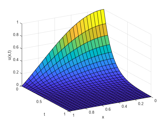
Create a surface plot of the solution. Since the problem is posed with cylindrical coordinates on a disc, the x values show the temperature on the disc some distance from the center, and the t values show how the temperature at a particular location changes over time.
surf(x,t,u)
xlabel('x')
ylabel('t')
zlabel('u(x,t)')
view([150 25])
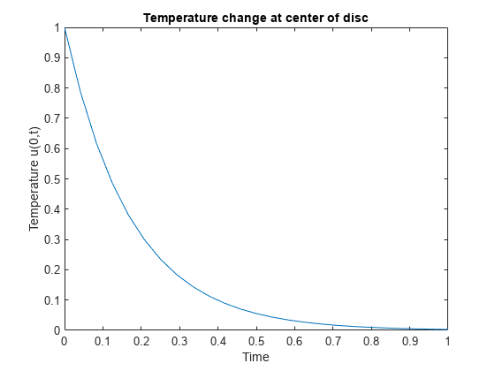
Plot the temperature change at the center () of the disc.
plot(t,sol(:,1))
xlabel('Time')
ylabel('Temperature u(0,t)')
title('Temperature change at center of disc')
Local Functions
Listed here are the local helper functions that the PDE solver pdepe calls to calculate the solution. Alternatively, you can save these functions as their own files in a directory on the MATLAB path.
function [c,f,s] = heatcyl(x,t,u,dudx)
c = 1;
f = dudx;
s = 0;
end
%----------------------------------------------
function u0 = heatic(x)
n = 2.404825557695773;
u0 = besselj(0,n*x);
end
%----------------------------------------------
function [pl,ql,pr,qr] = heatbc(xl,ul,xr,ur,t)
n = 2.404825557695773;
pl = 0; %ignored by solver since m=1
ql = 0; %ignored by solver since m=1
pr = ur-besselj(0,n)*exp(-n^2*t);
qr = 0;
end
%----------------------------------------------
Solve Oscillatory PDE with Event Logging
Solve a partial differential equation and use an event function to log zero-crossings in the oscillatory solution.
Consider the equation
The equation is defined for and . The initial condition is
The boundary conditions are
Additionally, the zero-crossings of the solution are of interest.
To solve this equation in MATLAB, you need to code the equation, initial conditions, boundary conditions, and event function, then select a suitable solution mesh before calling the solver pdepe. You either can include the required functions as local functions at the end of a file (as done here), or save them as separate, named files in a directory on the MATLAB path.
Code Equation
Before you can code the equation, you need to rewrite it in a form that the pdepe solver expects. The standard form that pdepe expects is
The PDE equation is already in this form:
So you can read off the relevant terms:
Now you can create a function to code the equation. The function should have the signature [c,f,s] = oscpde(x,t,u,dudx):
xis the independent spatial variable.tis the independent time variable.uis the dependent variable being differentiated with respect toxandt.dudxis the partial spatial derivative .The outputs
c,f, andscorrespond to coefficients in the standard PDE equation form expected bypdepe. These coefficients are coded in terms of the input variablesx,t,u, anddudx.
As a result, the equation in this example can be represented by the function:
function [c,f,s] = oscpde(x,t,u,dudx)
c = 1/x;
f = u/t;
s = 0;
end
(Note: All functions are included as local functions at the end of the example.)
Code Initial Conditions
Next, write a function that returns the initial condition. The initial condition is applied at the first time value tspan(1). The function should have the signature u0 = oscic(x).
The corresponding function for is
function u0 = oscic(x)
u0 = 1;
end
Code Boundary Conditions
Now, write a function that evaluates the boundary conditions
For problems posed on the interval , the boundary conditions apply for all and either or . The standard form for the boundary conditions expected by the solver is
Written in this form, the boundary conditions for this problem become
The boundary function should have the function signature [pl,ql,pr,qr] = oscbc(xl,ul,xr,ur,t):
The inputs
xlandulcorrespond to and for the left boundary.The inputs
xrandurcorrespond to and for the right boundary.tis the independent time variable.The outputs
plandqlcorrespond to and for the left boundary ( for this problem).The outputs
prandqrcorrespond to and for the right boundary ( for this problem).
The boundary conditions in this example are represented by the function:
function [pl,ql,pr,qr] = oscbc(xl,ul,xr,ur,t)
pl = ul - 1;
ql = 0;
pr = ur - cos(pi*t);
qr = 0;
end
Code Event Function
Use an event function to log the zero-crossings of the solution in the integration. The event function has a function signature of [value,isterminal,direction] = pdevents(m,t,xmesh,umesh):
mis the coordinate symmetry specified as the first input topdepe.tis the current time (a scalar).xmeshis the spatial mesh.umeshcontains the solution at the mesh points.valueis an equation of interest, usually expressed in terms of the solutionumesh. Whenvalueequals 0, an event occurs.isterminalspecifies whether an event stops the integration. Ifisterminalis 0, events are logged but the integration does not stop. Ifisterminalis 1, then the integration stops when an event occurs.directionspecifies the direction of zero crossing. If 1, only zero-crossings with a positive slope trigger an event. If -1, the zero-crossings must have a negative slope. If 0, then any zero-crossing triggers an event.
At each time in the integration, the solver calls the event function to check for zero crossings. To log all zero crossings, value should look for changes in sign in the solution vector umesh. Specify isterminal and direction as vectors of zeros with the same size, since the events in this example are not terminal and the zero-crossings can occur with any slope.
The event function for this problem is
function [value,isterminal,direction] = pdevents(m,t,xmesh,umesh)
value = umesh;
isterminal = zeros(size(umesh));
direction = zeros(size(umesh));
end
Select Solution Mesh
Before solving the equation you need to specify the mesh points at which you want pdepe to evaluate the solution. For this problem, use a fine mesh of 50 points in the intervals and . A fine mesh gives good resolution of the oscillatory solution.
x = linspace(0,1,50);
t = linspace(0.1,pi,50);
Solve Equation
Finally, solve the equation using the symmetry m, the PDE equation, the initial conditions, the boundary conditions, the event function, and the meshes for x and t. Use odeset to create an options structure that references the events function, and pass in the structure as the last input argument to pdepe. Specify five output arguments to return information from both the event function and the solver:
solis the solution computed bypdepe.tsolis a vector of times before a terminal event.tsolis equal totwhen no events are terminal.soleis the solution at the time of each event.teis the time of each event.ieis the index of each event. Sincevalues = umeshin the event function,iegives the indices ofumeshthat triggered an event at each time step.
m = 0;
options = odeset('Events',@pdevents);
[sol,tsol,sole,te,ie] = pdepe(m,@oscpde,@oscic,@oscbc,x,t,options);
Extract the solution as a matrix u.
u = sol(:,:,1);
Plot Solution
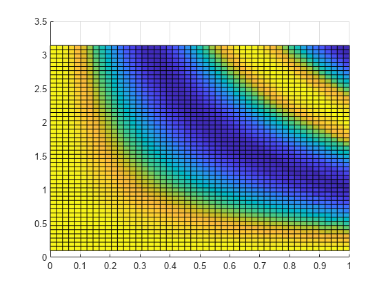
Create a surface plot of the solution and view the plot from above.
surf(x,t,u)
view(2)
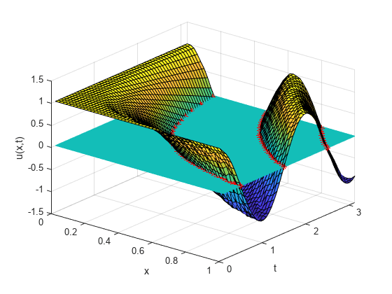
Plot the points where events occurred, with a surface for reference. The output index vector ie is useful to pick out the event locations. The expression x(ie)' gives the x-values where events occurred, and the expression sole(x==x(ie)') gives the corresponding solution values.
view([39 30])
xlabel('x')
ylabel('t')
zlabel('u(x,t)')
hold on
plot3(x(ie)',te,sole(x==x(ie)'),'r*')
surf(x,t,zeros(size(u)),'EdgeColor','flat')
hold off
Local Functions
Listed here are the local helper functions that the PDE solver pdepe calls to calculate the solution. Alternatively, you can save these functions as their own files in a directory on the MATLAB path.
function [c,f,s] = oscpde(x,t,u,dudx)
c = 1/x;
f = u/t;
s = 0;
end
%----------------------------------------------
function u0 = oscic(x)
u0 = 1;
end
%----------------------------------------------
function [pl,ql,pr,qr] = oscbc(xl,ul,xr,ur,t)
pl = ul - 1;
ql = 0;
pr = ur - cos(pi*t);
qr = 0;
end
%----------------------------------------------
function [value, isterminal, direction] = pdevents(m,t,xmesh,umesh)
value = umesh;
isterminal = zeros(size(umesh));
direction = zeros(size(umesh));
end
%----------------------------------------------
Input Arguments
Output Arguments
Tips
If
uji = sol(j,:,i)approximates componentiof the solution at timetspan(j)and mesh pointsxmesh, thenpdevalevaluates the approximation and its partial derivative ∂ui/∂x at the array of pointsxoutand returns them inuoutandduoutdx:[uout,duoutdx] = pdeval(m,xmesh,uji,xout). Thepdevalfunction evaluates the partial derivative ∂ui/∂x rather than the flux. The flux is continuous, but at a material interface the partial derivative may have a jump.
Algorithms
The time integration is done with the ode15s solver. pdepe exploits the capabilities of
ode15s for solving the differential-algebraic equations that arise when
the PDE contains elliptic equations, and for handling Jacobians with a specified sparsity
pattern.
After discretization, elliptic equations give rise to algebraic equations. If the elements
of the initial-conditions vector that correspond to elliptic equations are not consistent with
the discretization, pdepe tries to adjust them before beginning the time
integration. For this reason, the solution returned for the initial time may have a
discretization error comparable to that at any other time. If the mesh is sufficiently fine,
pdepe can find consistent initial conditions close to the given ones.
If pdepe displays a message that it has difficulty finding consistent
initial conditions, try refining the mesh. No adjustment is necessary for elements of the
initial conditions vector that correspond to parabolic equations.
References
[1] Skeel, R. D. and M. Berzins, "A Method for the Spatial Discretization of Parabolic Equations in One Space Variable," SIAM Journal on Scientific and Statistical Computing, Vol. 11, 1990, pp.1–32.
Extended Capabilities
Version History
Introduced before R2006a
You can also select a web site from the following list:
Americas
- América Latina (Español)
- Canada (English)
- United States (English)
Europe
- Belgium (English)
- Denmark (English)
- Deutschland (Deutsch)
- España (Español)
- Finland (English)
- France (Français)
- Ireland (English)
- Italia (Italiano)
- Luxembourg (English)
- Netherlands (English)
- Norway (English)
- Österreich (Deutsch)
- Portugal (English)
- Sweden (English)
- Switzerland
- United Kingdom (English)