polyval
Polynomial evaluation
Description
y = polyval(p,x)p at each point in x.
The argument p is a vector of length n+1 whose
elements are the coefficients (in descending powers) of an
nth-degree polynomial:
The polynomial coefficients in p can be calculated for
different purposes by functions like polyint, polyder, and polyfit, but you can specify any
vector for the coefficients.
To evaluate a polynomial in a matrix sense, use polyvalm instead.
y = polyval(p,x,[],mu)[
use the optional output y,delta]
= polyval(p,x,S,mu)mu produced by polyfit to center and scale the
data. mu(1) is mean(x), and
mu(2) is std(x). Using these values,
polyval centers x at zero and scales it to
have unit standard deviation,
This centering and scaling transformation improves the numerical properties of the polynomial.
Examples
Evaluate Polynomial at Several Points
Evaluate the polynomial at the points . The polynomial coefficients can be represented by the vector [3 2 1].
p = [3 2 1];
x = [5 7 9];
y = polyval(p,x)
y = 1×3

    86   162   262
Integrate Quartic Polynomial
Evaluate the definite integral
Create a vector to represent the polynomial integrand . The term is absent and thus has a coefficient of 0.
p = [3 0 -4 10 -25];
Use polyint to integrate the polynomial using a constant of integration equal to 0.
q = polyint(p)
q = 1×6

    0.6000         0   -1.3333    5.0000  -25.0000         0
Find the value of the integral by evaluating q at the limits of integration.
a = -1;
b = 3;
I = diff(polyval(q,[a b]))
I = 49.0667
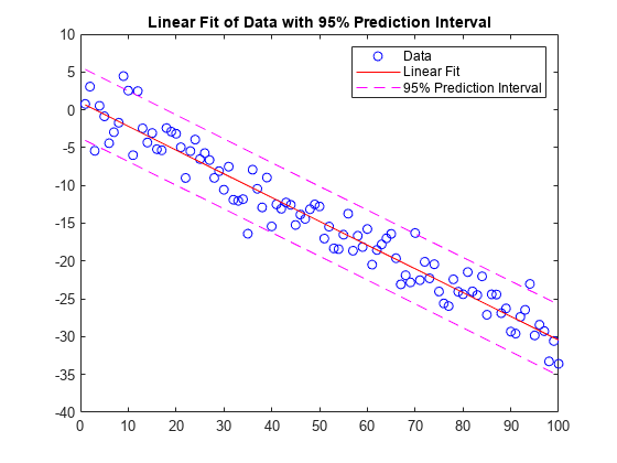
Linear Regression with Error Estimate
Fit a linear model to a set of data points and plot the results, including an estimate of a 95% prediction interval.
Create a few vectors of sample data points (x,y). Use polyfit to fit a first degree polynomial to the data. Specify two outputs to return the coefficients for the linear fit as well as the error estimation structure.
x = 1:100;
y = -0.3*x + 2*randn(1,100);
[p,S] = polyfit(x,y,1)
p = 1×2

   -0.3142    0.9614
S = struct with fields:
           R: [2x2 double]
          df: 98
       normr: 22.7673
    rsquared: 0.9407
Evaluate the first-degree polynomial fit in p at the points in x. Specify the error estimation structure as the third input so that polyval calculates an estimate of the standard error. The standard error estimate is returned in delta.
[y_fit,delta] = polyval(p,x,S);
Plot the original data, linear fit, and 95% prediction interval .
plot(x,y,'bo')
hold on
plot(x,y_fit,'r-')
plot(x,y_fit+2*delta,'m--',x,y_fit-2*delta,'m--')
title('Linear Fit of Data with 95% Prediction Interval')
legend('Data','Linear Fit','95% Prediction Interval')
Use Centering and Scaling to Improve Numerical Properties
Create a table of population data for the years 1750 - 2000 and plot the data points.
year = (1750:25:2000)';
pop = 1e6*[791 856 978 1050 1262 1544 1650 2532 6122 8170 11560]';
T = table(year, pop)
T=11×2 table
    year       pop
    ____    _________

    1750     7.91e+08
    1775     8.56e+08
    1800     9.78e+08
    1825     1.05e+09
    1850    1.262e+09
    1875    1.544e+09
    1900     1.65e+09
    1925    2.532e+09
    1950    6.122e+09
    1975     8.17e+09
    2000    1.156e+10
plot(year,pop,'o')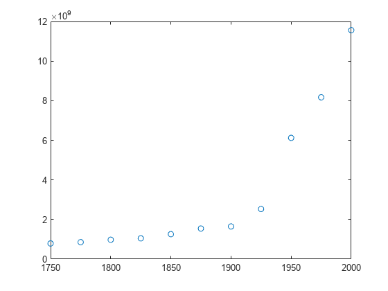
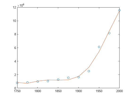
Use polyfit with three outputs to fit a 5th-degree polynomial using centering and scaling, which improves the numerical properties of the problem. polyfit centers the data in year at 0 and scales it to have a standard deviation of 1, which avoids an ill-conditioned Vandermonde matrix in the fit calculation.
[p,~,mu] = polyfit(T.year, T.pop, 5);
Use polyval with four inputs to evaluate p with the scaled years, (year-mu(1))/mu(2). Plot the results against the original years.
f = polyval(p,year,[],mu);
hold on
plot(year,f)
hold off
Input Arguments
Output Arguments
Extended Capabilities
Version History
Introduced before R2006a
See Also
You can also select a web site from the following list:
Americas
- América Latina (Español)
- Canada (English)
- United States (English)
Europe
- Belgium (English)
- Denmark (English)
- Deutschland (Deutsch)
- España (Español)
- Finland (English)
- France (Français)
- Ireland (English)
- Italia (Italiano)
- Luxembourg (English)
- Netherlands (English)
- Norway (English)
- Österreich (Deutsch)
- Portugal (English)
- Sweden (English)
- Switzerland
- United Kingdom (English)