surfnorm
Surface normals
Description
surfnorm(
creates a three-dimensional surface plot and displays its surface normals. A
surface normal is the imaginary line perpendicular to a flat surface, or
perpendicular to the tangent plane at a point on a non-flat surface.X,Y,Z)
The function plots the values in matrix Z as heights above
a grid in the x-y plane defined by
X and Y. The color of the surface
varies according to the heights specified by Z. The matrices
X, Y, and Z must be
the same size.
surfnorm( creates a surface with
normals and uses the column and row indices of the elements in
Z)Z as the x and
y-coordinates, respectively.
surfnorm( plots
into the axes specified by ax,___)ax instead of the current axes.
Specify the axes as the first input argument.
surfnorm(___,
specifies surface properties using one or more name-value pair arguments. For
example, Name,Value)'FaceAlpha',0.5 creates a semitransparent
surface.
Examples
Create Surface Plot With Surface Normals
Create a cone. Then plot the data as a surface and display the surface normals. The surface uses Z for both height and color.
[X,Y,Z] = cylinder(1:10);
surfnorm(X,Y,Z)

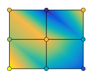
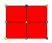
Modify Surface Plot Appearance
Create a surface with no edges by specifying the EdgeColor name-value pair with 'none' as the value.
[X,Y,Z] = cylinder(1:10);
surfnorm(X,Y,Z,'EdgeColor','none')

Light a Surface Using Surface Normals
Use the surface normals of a curved surface to light a flat surface.
First, display a flat surface.
surf(ones(49),'EdgeColor','none');

Display the curved surface to use as a lighting source.
surf(peaks);

Now, draw the flat surface again, this time with lighting from the curved surface. To do this, first calculate the surface normals of the curved surface.
[nx, ny, nz] = surfnorm(peaks);
Combine the x, y, and z surface normal components into a single 49-by-49-by-3 array.
b = reshape([nx ny nz], 49,49,3);
Create a flat surface again, this time supplying this array as a value for the VertexNormals property. MATLAB® uses the VertexNormals property to calculate the surface lighting. Set the lighting algorithm to gouraud and add a light using camlight.
surf(ones(49),'VertexNormals',b,'EdgeColor','none');
lighting gouraud
camlight

Input Arguments
X — x-coordinates
matrix
x-coordinates, specified as a matrix the same size as
Y and Z.
You can use the meshgrid function to create
the X and Y matrices.
The XData property of the Surface
object stores the x-coordinates.
Example: X = [1 2 3; 1 2 3; 1 2 3]
Example: [X,Y] = meshgrid(-5:0.5:5)
Data Types: single | double | int8 | int16 | int32 | int64 | uint8 | uint16 | uint32 | uint64
Y — y-coordinates
matrix
y-coordinates, specified as a matrix the same size as
X and Z.
You can use the meshgrid function to create
the X and Y matrices.
The YData property of the surface object stores the
y-coordinates.
Example: Y = [1 1 1; 2 2 2; 3 3 3]
Example: [X,Y] = meshgrid(-5:0.5:5)
Data Types: single | double | int8 | int16 | int32 | int64 | uint8 | uint16 | uint32 | uint64
Z — z-coordinates
matrix
z-coordinates, specified as a matrix.
Z must have at least three rows and three columns.
Z also sets the surface colors.
The ZData property of the surface object stores the
z-coordinates.
Example: Z = [1 2 3; 4 5 6; 7 8 9]
Data Types: single | double | int8 | int16 | int32 | int64 | uint8 | uint16 | uint32 | uint64
ax — Axes to plot in
axes object
Axes to plot in, specified as an axes object. If you do
not specify the axes, then surfnorm plots into the
current axes.
Name-Value Arguments
Specify optional pairs of arguments as
Name1=Value1,...,NameN=ValueN, where Name is
the argument name and Value is the corresponding value.
Name-value arguments must appear after other arguments, but the order of the
pairs does not matter.
Before R2021a, use commas to separate each name and value, and enclose
Name in quotes.
Example: surfnorm(X,Y,Z,'FaceAlpha',0.5,'EdgeColor','none')
creates a semitransparent surface with no edges drawn.
Note
The properties listed here are only a subset. For a full list, see Surface Properties.
Edge line color, specified as one of the values listed here.
The default color of [0 0 0] corresponds to black
edges.
| Value | Description |
|---|---|
'none' | Do not draw the edges. |
'flat' | Use a different color for each edge based on the values
in the
|
'interp' |
Use interpolated coloring for each edge based on the values in the
|
| RGB triplet, hexadecimal color code, or color name |
Use the specified color for all the edges. This option does not use the color
values in the
|
RGB triplets and hexadecimal color codes are useful for specifying custom colors.
An RGB triplet is a three-element row vector whose elements specify the intensities of the red, green, and blue components of the color. The intensities must be in the range
[0,1]; for example,[0.4 0.6 0.7].A hexadecimal color code is a character vector or a string scalar that starts with a hash symbol (
#) followed by three or six hexadecimal digits, which can range from0toF. The values are not case sensitive. Thus, the color codes"#FF8800","#ff8800","#F80", and"#f80"are equivalent.
Alternatively, you can specify some common colors by name. This table lists the named color options, the equivalent RGB triplets, and hexadecimal color codes.
| Color Name | Short Name | RGB Triplet | Hexadecimal Color Code | Appearance |
|---|---|---|---|---|
"red" | "r" | [1 0 0] | "#FF0000" |
|
"green" | "g" | [0 1 0] | "#00FF00" |
|
"blue" | "b" | [0 0 1] | "#0000FF" |
|
"cyan"
| "c" | [0 1 1] | "#00FFFF" |
|
"magenta" | "m" | [1 0 1] | "#FF00FF" |
|
"yellow" | "y" | [1 1 0] | "#FFFF00" |
|
"black" | "k" | [0 0 0] | "#000000" |
|
"white" | "w" | [1 1 1] | "#FFFFFF" |
|
Here are the RGB triplets and hexadecimal color codes for the default colors MATLAB® uses in many types of plots.
| RGB Triplet | Hexadecimal Color Code | Appearance |
|---|---|---|
[0 0.4470 0.7410] | "#0072BD" |
|
[0.8500 0.3250 0.0980] | "#D95319" |
|
[0.9290 0.6940 0.1250] | "#EDB120" |
|
[0.4940 0.1840 0.5560] | "#7E2F8E" |
|
[0.4660 0.6740 0.1880] | "#77AC30" |
|
[0.3010 0.7450 0.9330] | "#4DBEEE" |
|
[0.6350 0.0780 0.1840] | "#A2142F" |
|
Line style, specified as one of the options listed in this table.
| Line Style | Description | Resulting Line |
|---|---|---|
"-" | Solid line |
|
"--" | Dashed line |
|
":" | Dotted line |
|
"-." | Dash-dotted line |
|
"none" | No line | No line |
Face color, specified as one of the values in this table.
| Value | Description |
|---|---|
'flat' | Use a different color for each face based on the values
in the
|
'interp' |
Use interpolated coloring for each face based on the values in the
|
| RGB triplet, hexadecimal color code, or color name |
Use the specified color for all the faces. This option does not use the color
values in the
|
'texturemap' | Transform the color data in CData so that
it conforms to the surface. |
'none' | Do not draw the faces. |
RGB triplets and hexadecimal color codes are useful for specifying custom colors.
An RGB triplet is a three-element row vector whose elements specify the intensities of the red, green, and blue components of the color. The intensities must be in the range
[0,1]; for example,[0.4 0.6 0.7].A hexadecimal color code is a character vector or a string scalar that starts with a hash symbol (
#) followed by three or six hexadecimal digits, which can range from0toF. The values are not case sensitive. Thus, the color codes"#FF8800","#ff8800","#F80", and"#f80"are equivalent.
Alternatively, you can specify some common colors by name. This table lists the named color options, the equivalent RGB triplets, and hexadecimal color codes.
| Color Name | Short Name | RGB Triplet | Hexadecimal Color Code | Appearance |
|---|---|---|---|---|
"red" | "r" | [1 0 0] | "#FF0000" |
|
"green" | "g" | [0 1 0] | "#00FF00" |
|
"blue" | "b" | [0 0 1] | "#0000FF" |
|
"cyan"
| "c" | [0 1 1] | "#00FFFF" |
|
"magenta" | "m" | [1 0 1] | "#FF00FF" |
|
"yellow" | "y" | [1 1 0] | "#FFFF00" |
|
"black" | "k" | [0 0 0] | "#000000" |
|
"white" | "w" | [1 1 1] | "#FFFFFF" |
|
Here are the RGB triplets and hexadecimal color codes for the default colors MATLAB uses in many types of plots.
| RGB Triplet | Hexadecimal Color Code | Appearance |
|---|---|---|
[0 0.4470 0.7410] | "#0072BD" |
|
[0.8500 0.3250 0.0980] | "#D95319" |
|
[0.9290 0.6940 0.1250] | "#EDB120" |
|
[0.4940 0.1840 0.5560] | "#7E2F8E" |
|
[0.4660 0.6740 0.1880] | "#77AC30" |
|
[0.3010 0.7450 0.9330] | "#4DBEEE" |
|
[0.6350 0.0780 0.1840] | "#A2142F" |
|
Output Arguments
Tips
To reverse the direction of the normals, call
surfnormwith transposed arguments:surfnorm(X',Y',Z')
To show the direction of the normals on a surface, use the
surfnormfunction to calculate the surface normals and then thequiver3function to display them.[Nx,Ny,Nz] = surfnorm(X,Y,Z); quiver3(X,Y,Z,Nx,Ny,Nz)
The surface normals represent conditions at vertices and are not normalized. Normals for surface elements that face away from the viewer are not visible.
Algorithms
surfnorm uses bicubic interpolation in the x,
y, and z directions to calculate the surface
normals of the data. To allow for interpolation at the boundaries, the function uses
quadratic extrapolation to expand the data. After performing the bicubic fit of the
data, diagonal vectors are computed and crossed to form the normal at each
vertex.
Version History
Introduced before R2006a
You can also select a web site from the following list:
Americas
- América Latina (Español)
- Canada (English)
- United States (English)
Europe
- Belgium (English)
- Denmark (English)
- Deutschland (Deutsch)
- España (Español)
- Finland (English)
- France (Français)
- Ireland (English)
- Italia (Italiano)
- Luxembourg (English)
- Netherlands (English)
- Norway (English)
- Österreich (Deutsch)
- Portugal (English)
- Sweden (English)
- Switzerland
- United Kingdom (English)