Geometric Distribution
Overview
The geometric distribution is a one-parameter family of curves that models the number of failures before one success in a series of independent trials, where each trial results in either success or failure, and the probability of success in any individual trial is constant. For example, if you toss a coin, the geometric distribution models the number of tails observed before the result is heads. The geometric distribution is discrete, existing only on the nonnegative integers.
Statistics and Machine Learning Toolbox™ offers multiple ways to work with the geometric distribution.
Use distribution-specific functions (
geocdf,geopdf,geoinv,geostat,geornd) with specified distribution parameters. The distribution-specific functions can accept parameters of multiple geometric distributions.Use generic distribution functions (
cdf,icdf,pdf,mle,random) with a specified distribution name ('Geometric') and parameters.
Parameters
The geometric distribution uses the following parameter.
| Parameter | Description | Support |
|---|---|---|
p | Probability of success |
Probability Density Function
The probability density function (pdf) of the geometric distribution is
where p is the probability of success, and x is the number of failures before the first success. The result y is the probability of observing exactly x trials before a success, when the probability of success in any given trial is p. For discrete distributions, the pdf is also known as the probability mass function (pmf).
For an example, see Compute Geometric Distribution pdf.
Cumulative Distribution Function
The cumulative distribution function (cdf) of the geometric distribution is
where p is the probability of success, and x is the number of failures before the first success. The result y is the probability of observing up to x trials before a success, when the probability of success in any given trial is p.
For an example, see Compute Geometric Distribution cdf.
Descriptive Statistics
The mean of the geometric distribution is and the variance of the geometric distribution is where p is the probability of success.
Hazard Function
The hazard function (instantaneous failure rate) is the ratio of the pdf and the complement of the cdf. If f(t) and F(t) are the pdf and cdf of a distribution (respectively), then the hazard rate is . Substituting the pdf and cdf of the geometric distribution for f(t) and F(t) above yields a constant equal to the reciprocal of the mean. The geometric distribution is the only discrete distribution with constant hazard function. Consequently, the probability of observing a success is independent of the number of failures already observed.
Examples
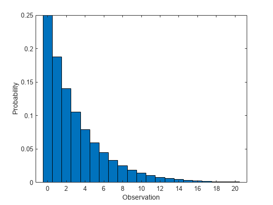
Compute Geometric Distribution pdf
Compute the pdf of the geometric distribution with the probability of success 0.25.
x = 0:20;
y = geopdf(x,0.25);
Plot the pdf with bars of width 1.
figure
bar(x,y,1)
xlabel('Observation')
ylabel('Probability')
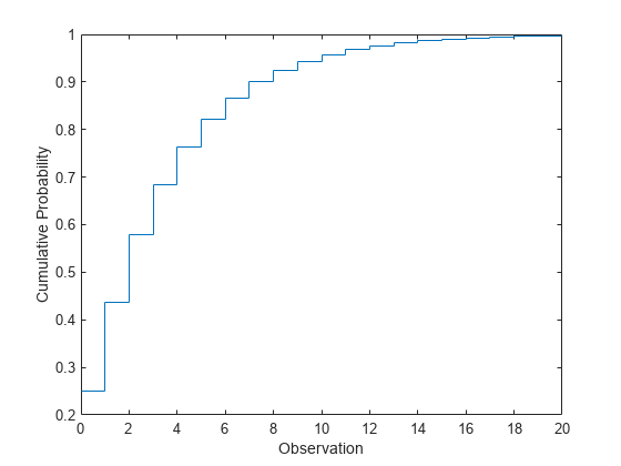
Compute Geometric Distribution cdf
Compute the cdf of the geometric distribution with the probability of success 0.25.
x = 0:20;
y = geocdf(x,0.25);
Plot the cdf.
figure
stairs(x,y)
xlabel('Observation')
ylabel('Cumulative Probability')
Compute Geometric Distribution Probabilities
Assume that the probability of a five-year-old car battery not starting in cold weather is 0.03. The driver attempts to start the car every morning during a span of cold weather lasting 25 days. Model this scenario with a geometric distribution, where the event to observe is the car not starting.
Compute the cdf of 25 to find the probability of the car not starting during one of the 25 days.
x = 25;
p = 0.03;
notstart = geocdf(x,p)
notstart = 0.5470
Compute the complement to find the probability of the car starting every day for all 25 days.
start = 1 - notstart
start = 0.4530
Related Distributions
Exponential Distribution — The exponential distribution is a one-parameter continuous distribution that has parameter μ (mean). The exponential distribution is a continuous analog of the geometric and is the only distribution other than geometric with a constant hazard function.
Negative Binomial Distribution — The negative binomial distribution is a two-parameter discrete distribution that has parameters r and p, and models the number of failures observed before r successes with probability p of success in a single trial. The geometric distribution occurs as the negative binomial distribution with r = 1.
References
[1] Abramowitz, Milton, and Irene A. Stegun, eds. Handbook of Mathematical Functions: With Formulas, Graphs, and Mathematical Tables. 9. Dover print.; [Nachdr. der Ausg. von 1972]. Dover Books on Mathematics. New York, NY: Dover Publ, 2013.
[2] Devroye, Luc. Non-Uniform Random Variate Generation. New York, NY: Springer New York, 1986. https://doi.org/10.1007/978-1-4613-8643-8
[3] Evans, Merran, Nicholas Hastings, and Brian Peacock. Statistical Distributions. 2nd ed. New York: J. Wiley, 1993.
See Also
geocdf | geopdf | geoinv | geostat | geornd | NegativeBinomialDistribution
Related Topics
You can also select a web site from the following list:
Americas
- América Latina (Español)
- Canada (English)
- United States (English)
Europe
- Belgium (English)
- Denmark (English)
- Deutschland (Deutsch)
- España (Español)
- Finland (English)
- France (Français)
- Ireland (English)
- Italia (Italiano)
- Luxembourg (English)
- Netherlands (English)
- Norway (English)
- Österreich (Deutsch)
- Portugal (English)
- Sweden (English)
- Switzerland
- United Kingdom (English)