Negative Loglikelihood Functions
Negative loglikelihood functions for supported Statistics and Machine Learning Toolbox™ distributions all end with like, as in explike. Each function represents a parametric family of distributions.
Input arguments are lists of parameter values specifying a particular member of the
distribution family followed by an array of data. Functions return the negative
loglikelihood of the parameters, given the data.
To find maximum likelihood estimates (MLEs), you can use a negative loglikelihood
function as an objective function of the optimization problem and solve it by using the
MATLAB® function fminsearch or functions in Optimization Toolbox™ and Global Optimization Toolbox. These functions allow you to choose a search algorithm and exercise
low-level control over algorithm execution. By contrast, the mle function and the distribution fitting functions that end with
fit, such as normfit and gamfit, use preset algorithms with
options limited to those set by the statset function.
You can specify a parametric family of distributions by using the probability density function (pdf) f(x|θ), where x represents an outcome of a random variable and θ represents the distribution parameters. When you view f(x|θ) as a function of θ for a fixed x, the function f(x|θ) is the likelihood of parameters θ for a single outcome x. The likelihood of parameters θ for an independent and identically distributed random sample data set X is:
Given X, MLEs maximize L(θ) over all possible θ. Numerical algorithms find MLEs that (equivalently) maximize the loglikelihood function, log(L(θ)). The logarithm transforms the product of potentially small likelihoods into a sum of logs, which is easier to distinguish from 0 in computation. For convenience, Statistics and Machine Learning Toolbox negative loglikelihood functions return the negative of this sum because optimization algorithms typically search for minima rather than maxima.
Find MLEs Using Negative Loglikelihood Function
This example shows how to find MLEs by using the gamlike and fminsearch functions.
Use the gamrnd function to generate a random sample from a specific Gamma Distribution.
rng default;  % For reproducibility
a = [1,2];
X = gamrnd(a(1),a(2),1e3,1);
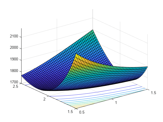
Visualize the likelihood surface in the neighborhood of a given X by using the gamlike function.
mesh = 50;
delta = 0.5;
a1 = linspace(a(1)-delta,a(1)+delta,mesh);
a2 = linspace(a(2)-delta,a(2)+delta,mesh);
logL = zeros(mesh); % Preallocate memory
for i = 1:mesh
    for j = 1:mesh
        logL(i,j) = gamlike([a1(i),a2(j)],X);
    end
end

[A1,A2] = meshgrid(a1,a2);
surfc(A1,A2,logL)
Search for the minimum of the likelihood surface by using the fminsearch function.
LL = @(u)gamlike([u(1),u(2)],X); % Likelihood given X
MLES = fminsearch(LL,[1,2])
MLES = 1×2
0.9980 2.0172
Compare MLES to the estimates returned by the gamfit function.
ahat = gamfit(X)
ahat = 1×2

    0.9980    2.0172
The difference of each parameter between MLES and ahat is less than 1e-4.
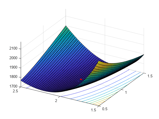
Add the MLEs to the surface plot.
hold on
plot3(MLES(1),MLES(2),LL(MLES),'ro','MarkerSize',5,'MarkerFaceColor','r')
view([-60 40]) % Rotate to show the minimum
See Also
negloglik | statset | fminsearch | surfc
Related Topics
You can also select a web site from the following list:
Americas
- América Latina (Español)
- Canada (English)
- United States (English)
Europe
- Belgium (English)
- Denmark (English)
- Deutschland (Deutsch)
- España (Español)
- Finland (English)
- France (Français)
- Ireland (English)
- Italia (Italiano)
- Luxembourg (English)
- Netherlands (English)
- Norway (English)
- Österreich (Deutsch)
- Portugal (English)
- Sweden (English)
- Switzerland
- United Kingdom (English)