Student's t Distribution
Overview
The Student’s t distribution is a one-parameter family of curves. This distribution is typically used to test a hypothesis regarding the population mean when the population standard deviation is unknown.
Statistics and Machine Learning Toolbox™ offers multiple ways to work with the Student’s t distribution.
Use distribution-specific functions (
tcdf,tinv,tpdf,trnd,tstat) with specified distribution parameters. The distribution-specific functions can accept parameters of multiple Student’s t distributions.Use generic distribution functions (
cdf,icdf,pdf,random) with a specified distribution name ('T') and parameters.
Parameters
The Student’s t distribution uses the following parameter.
| Parameter | Description | Support |
|---|---|---|
| nu (ν) | Degrees of freedom | ν = 1, 2, 3,... |
Probability Density Function
The pdf of the Student's t distribution is
where ν is the degrees of freedom and Γ( · ) is the Gamma function. The result y is the probability of observing a particular value of x from the Student’s t distribution with ν degrees of freedom.
For an example, see Compute and Plot Student's t Distribution pdf.
Cumulative Distribution Function
The cdf of the Student’s t distribution is
where ν is the degrees of freedom and Γ( · ) is the Gamma function. The result p is the probability that a single observation from the t distribution with ν degrees of freedom falls in the interval [–∞, x].
For an example, see Compute and Plot Student's t Distribution cdf.
Inverse Cumulative Distribution Function
The t inverse function is defined in terms of the Student's t cdf as
where
ν is the degrees of freedom, and Γ( · ) is the Gamma function. The result x is the solution of the integral equation where you supply the probability p.
For an example, see Compute Student's t icdf.
Descriptive Statistics
The mean of the Student’s t distribution is μ = 0 for degrees of freedom ν greater than 1. If ν equals 1, then the mean is undefined.
The variance of the Student’s t distribution is for degrees of freedom ν greater than 2. If ν is less than or equal to 2, then the variance is undefined.
Examples
Compute and Plot Student's t Distribution pdf
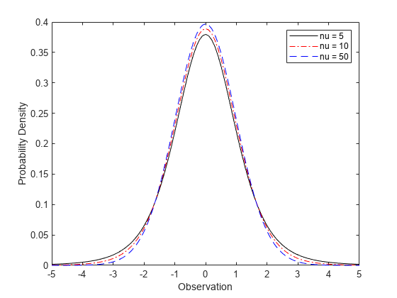
Compute the pdf of a Student's t distribution with degrees of freedom equal to 5, 10, and 50.
x = [-5:.1:5];
y1 = tpdf(x,5);
y2 = tpdf(x,10);
y3 = tpdf(x,50);
Plot the pdf for all three choices nu on the same axis.
figure;
plot(x,y1,'Color','black','LineStyle','-')
hold on
plot(x,y2,'Color','red','LineStyle','-.')
plot(x,y3,'Color','blue','LineStyle','--')
xlabel('Observation')
ylabel('Probability Density')
legend({'nu = 5','nu = 10','nu = 50'})
hold off
Compute and Plot Student's t Distribution cdf
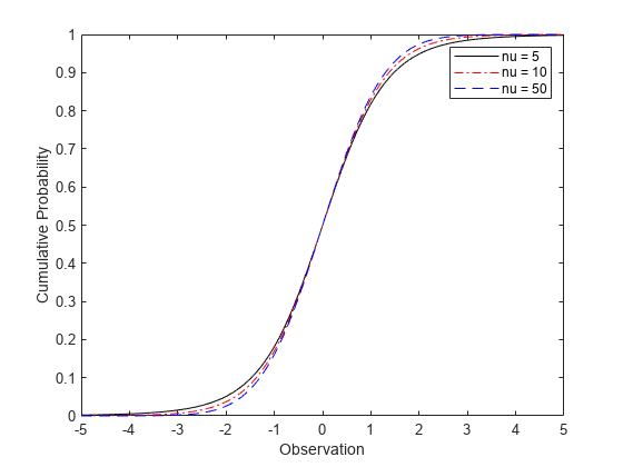
Compute the cdf of a Student's t distribution with degrees of freedom equal to 5, 10, and 50.
x = [-5:.1:5];
y1 = tcdf(x,5);
y2 = tcdf(x,10);
y3 = tcdf(x,50);
Plot the cdf for all three choices of nu on the same axis.
figure;
plot(x,y1,'Color','black','LineStyle','-')
hold on
plot(x,y2,'Color','red','LineStyle','-.')
plot(x,y3,'Color','blue','LineStyle','--')
xlabel('Observation')
ylabel('Cumulative Probability')
legend({'nu = 5','nu = 10','nu = 50'})
hold off
Compute Student's t icdf
Find the 95th percentile of the Student's t distribution with 50 degrees of freedom.
p = .95;
nu = 50;
x = tinv(p,nu)
x = 1.6759
Compare Student's t and Normal Distribution pdfs
The Student’s t distribution is a family of curves depending on a single parameter ν (the degrees of freedom). As the degrees of freedom ν approach infinity, the t distribution approaches the standard normal distribution.
Compute the pdfs for the Student's t distribution with the parameter nu = 5 and the Student's t distribution with the parameter nu = 15.
x = [-5:0.1:5];
y1 = tpdf(x,5);
y2 = tpdf(x,15);
Compute the pdf for a standard normal distribution.
z = normpdf(x,0,1);
Plot the Student's t pdfs and the standard normal pdf on the same figure.
plot(x,y1,'-.',x,y2,'--',x,z,'-')
legend('Student''s t Distribution with \nu=5', ...
    'Student''s t Distribution with \nu=15', ...
    'Standard Normal Distribution','Location','best')
xlabel('Observation')
ylabel('Probability Density')
title('Student''s t and Standard Normal pdfs')
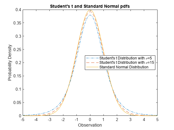
The standard normal pdf has shorter tails than the Student's t pdfs.
Related Distributions
Beta Distribution — The beta distribution is a two-parameter continuous distribution that has parameters a (first shape parameter) and b (second shape parameter). If Y has a Student's t distribution with ν degrees of freedom, then has beta distribution with the shape parameters a = ν/2 and b = ν/2. This relationship is used to compute values of the t cdf and inverse functions, and to generate t distributed random numbers.
Cauchy Distribution — The Cauchy distribution is a two-parameter continuous distribution with the parameters γ (scale) and δ (location). It is a special case of the Stable Distribution with the shape parameters α = 1 and β = 0. The standard Cauchy distribution (unit scale and location zero) is the Student’s t distribution with degrees of freedom ν equal to 1. The standard Cauchy distribution has an undefined mean and variance.
For an example, see Generate Cauchy Random Numbers Using Student's t.
Chi-Square Distribution — The chi-square distribution is a one-parameter continuous distribution that has the parameter ν (degrees of freedom). If Z has a standard normal distribution and χ2 has a chi-square distribution with degrees of freedom ν, then has a Student's t distribution with degrees of freedom ν.
Noncentral t Distribution — The noncentral t distribution is a two-parameter continuous distribution that generalizes the Student's t distribution and has the parameters ν (degrees of freedom) and δ (noncentrality). Setting δ = 0 yields the Student's t distribution.
Normal Distribution — The normal distribution is a two-parameter continuous distribution with the parameters μ (mean) and σ (standard deviation).
As the degrees of freedom ν approach infinity, the Student's t distribution approaches the standard normal distribution (zero mean and unit standard deviation).
For an example, see Compare Student's t and Normal Distribution pdfs
If x is a random sample of size n from a normal distribution with mean μ, then the statistic , where is the sample mean and s is the sample standard deviation, has a Student's t distribution with n —1 degrees of freedom.
For an example, see Compute Student's t Distribution cdf.
t Location-Scale Distribution — The t location-scale distribution is a three-parameter continuous distribution with the parameters μ (mean), σ (scale), and ν (shape). If x has a t location-scale distribution with the parameters µ, σ, and ν, then has a Student's t distribution with ν degrees of freedom.
References
[1] Abramowitz, Milton, and Irene A. Stegun, eds. Handbook of Mathematical Functions: With Formulas, Graphs, and Mathematical Tables. 9. Dover print.; [Nachdr. der Ausg. von 1972]. Dover Books on Mathematics. New York, NY: Dover Publ, 2013.
[2] Devroye, Luc. Non-Uniform Random Variate Generation. New York, NY: Springer New York, 1986. https://doi.org/10.1007/978-1-4613-8643-8
[3] Evans, Merran, Nicholas Hastings, and Brian Peacock. Statistical Distributions. 2nd ed. New York: J. Wiley, 1993.
[4] Kreyszig, Erwin. Introductory Mathematical Statistics: Principles and Methods. New York: Wiley, 1970.
See Also
tcdf | tpdf | tinv | tstat | trnd | ttest | ttest2
Related Topics
You can also select a web site from the following list:
Americas
- América Latina (Español)
- Canada (English)
- United States (English)
Europe
- Belgium (English)
- Denmark (English)
- Deutschland (Deutsch)
- España (Español)
- Finland (English)
- France (Français)
- Ireland (English)
- Italia (Italiano)
- Luxembourg (English)
- Netherlands (English)
- Norway (English)
- Österreich (Deutsch)
- Portugal (English)
- Sweden (English)
- Switzerland
- United Kingdom (English)