deconv
Least-squares deconvolution and polynomial division
Description
Polynomial Long Division
[ deconvolves a
vector x,r] =
deconv(y,h)h out of a vector y using
polynomial long division, and returns the quotient x and
remainder r such that y = conv(x,h) + r.
If y and h are vectors of polynomial
coefficients, then deconvolving them is equivalent to dividing the polynomial
represented by y by the polynomial represented by
h.
Least-Squares Deconvolution
Since R2023b
[
specifies the subsections of the convolved signal x,r] =
deconv(y,h,shape)y, where
y = conv(x,h,shape) + r.
If you use the least-squares deconvolution method
(Method="least-squares"), then you can specify
shape as "full",
"same", or "valid". Otherwise, if you
use the default long-division deconvolution method
(Method="long-division"), then shape
must be "full".
[ specifies options
using one or more name-value arguments in addition to any of the input argument
combinations in previous syntaxes.x,r] =
deconv(___,Name=Value)
You can specify the deconvolution method using
deconv(__,Method=algorithm), wherealgorithmcan be"long-division"or"least-squares".You can also specify the Tikhonov regularization factor to the least-squares solution of the deconvolution method using
deconv(__,RegularizationFactor=alpha).
Examples
Polynomial Division
Create two vectors, y and h, containing the coefficients of the polynomials and , respectively. Divide the first polynomial by the second by deconvolving h out of y. The deconvolution results in quotient coefficients corresponding to the polynomial and remainder coefficients corresponding to .
y = [2 7 4 9];
h = [1 0 1];
[x,r] = deconv(y,h)
x = 1×2

     2     7
r = 1×4

     0     0     2     2
Least-Squares Deconvolution of Fully Convolved Signal
Since R2023b
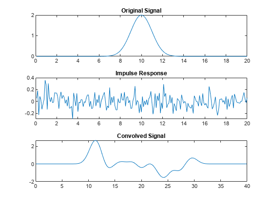
Create a signal x that has a Gaussian shape. Convolve this signal with an impulse response h that consists of random noise.
N = 200;
n = 0.1*(1:N);

rng("default")
x = 2*exp(-0.5*((n-10)).^2);
h = 0.1*randn(1,length(x));
y = conv(x,h);
Plot the original signal, the impulse response, and the convolved signal.
figure
tiledlayout(3,1)
nexttile
plot(n,x)
title("Original Signal")
nexttile
plot(n,h)
title("Impulse Response")
nexttile
plot(0.1*(1:length(y)),y)
title("Convolved Signal")
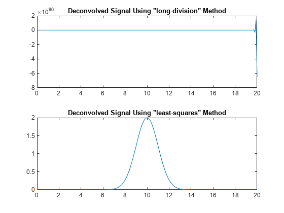
Next, find the deconvolution of signal y with respect to impulse response h using the default polynomial long-division method. Using this method, the deconvolution computation is unstable, and the result can rapidly increase.
[x1,r1] = deconv(y,h);
x1(end)
ans = 7.5992e+90
Instead, find the deconvolution using the least-squares method for a numerically stable computation.
[x2,r2] = deconv(y,h,Method="least-squares");Plot both deconvolution results. Here, the least-squares method correctly returns the original signal that has a Gaussian shape.
figure
tiledlayout(2,1)
nexttile
plot(n,x1)
title("Deconvolved Signal Using ""long-division"" Method")
nexttile
plot(n,x2)
title("Deconvolved Signal Using ""least-squares"" Method")
Least-Squares Deconvolution of Central Part of Convolved Signal
Since R2023b
Create two vectors. Find the central part of the convolution of xin and h that is the same size as xin. The central part of the convolved signal y has a length of 7 instead of the full length, which is length(xin)+length(h)-1, or 10.
xin = [-1 2 3 -2 0 1 2];
h = [2 4 -1 1];
y = conv(xin,h,"same")
y = 1×7
15 5 -9 7 6 7 -1
Find the least-squares deconvolution of signal y with respect to impulse response h. Use the "same" option to specify that the convolved signal y is only the central part, where y = conv(x,h,"same") + r. Show that deconv recovers the original signal in x within round-off error.
[x,r] = deconv(y,h,"same",Method="least-squares")
x = 1×7

   -1.0000    2.0000    3.0000   -2.0000    0.0000    1.0000    2.0000
r = 1×7
10-14 ×

         0    0.0888    0.1776         0         0         0         0
Least-Squares Deconvolution Problem with Infinite Solutions
Since R2023b
Create two vectors, each with two elements, and convolve them using the "valid" option. This option returns only those parts of the convolution that are computed without the zero-padded edges. In this case, the convolved signal y has only one element.
xin = [-1 2];
h = [2 5];
y = conv(xin,h,"valid")
y = -1
Find the least-squares deconvolution of convolved signal y with respect to impulse response h. With the "valid" option, deconv does not always return the original signal in x, but it returns the solution of the deconvolution problem that minimizes norm(x) instead.
[x,r] = deconv(y,h,"valid",Method="least-squares")
x = 1×2

   -0.1724   -0.0690
r = -3.3307e-16
To check the solution, you can find the full convolution of the computed signal x with h. The central part of this convolved signal is the same as the original y that defined the deconvolution problem.
yfull = conv(x,h,"full")yfull = 1×3
-0.3448 -1.0000 -0.3448
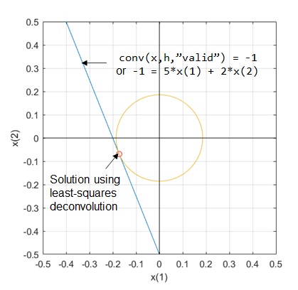
In this problem, deconv returns a different signal than the original signal because it solves for one equation with two variables, which is . This system is underdetermined, meaning this system has more variables than equations. This system has infinite solutions when using the least-squares method to minimize the residual norm, or norm(y - conv(x,h,"valid")), to 0. For this reason, deconv also finds a solution that minimizes norm(x).
The following figure illustrates the situation for this underdetermined problem. The blue line represents the infinite number of solutions to the equation . The orange circle represents the minimum distance from the origin to the line of solutions. The solution returned by deconv lies at the tangent point between the line and circle, indicating the solution closest to the origin.
Specify Regularization Factor for Noisy Signal
Since R2023b
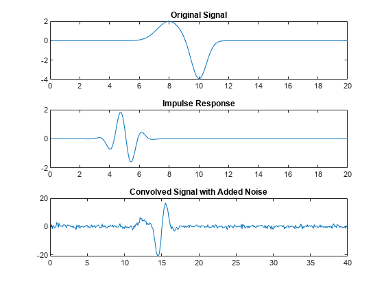
Create two signals, x and h, and convolve them. Add some random noise to the convolved signal in y.
N = 200;
n = 0.1*(1:N);

rng("default")
x = 2*exp(-0.8*(n - 8).^2) - 4*exp(-2*(n - 10).^2);
h = 2.*exp(-1*(n - 5).^2).*cos(4*n);
y = conv(x,h);
y = y + max(y)*0.05*randn(1,length(y));
Plot the original signal, the impulse response, and the convolved signal.
figure
tiledlayout(3,1)
nexttile
plot(n,x)
title("Original Signal")
nexttile
plot(n,h)
title("Impulse Response")
nexttile
plot(0.1*(1:length(y)),y)
title("Convolved Signal with Added Noise")
Next, find the deconvolution of the noisy signal y with respect to the impulse response h by using the least-squares method without a regularization factor. By default, the regularization factor is 0.
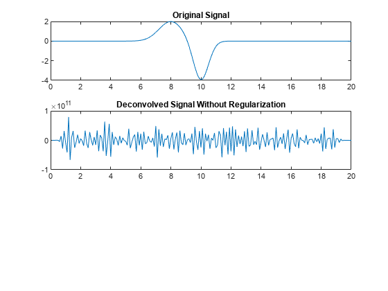
[x1,r1] = deconv(y,h,Method="least-squares");Plot the original signal and the deconvolved signal. Here, the deconv function without a regularization factor cannot recover the original signal from the noisy signal.
figure;
tiledlayout(3,1);
nexttile
plot(n,x)
title("Original Signal")
nexttile
plot(n,x1)
title("Deconvolved Signal Without Regularization");
Instead, find the deconvolution of y with respect to h by using the least-squares method with a regularization factor of 1. For an ill-conditioned deconvolution problem, such as one that involves noisy signal, you can specify a regularization factor so that overfitting does not occur in the least-squares solution.
[x2,r2] = deconv(y,h,Method="least-squares",RegularizationFactor=1);Plot this deconvolved signal. Here, the deconv function with a specified regularization factor recovers the original signal.
nexttile
plot(n,x2)
title("Deconvolved Signal Using Regularization")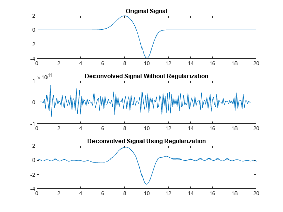
Input Arguments
Output Arguments
References
[1] Nagy, James G. “Fast Inverse QR Factorization for Toeplitz Matrices.” SIAM Journal on Scientific Computing 14, no. 5 (September 1993): 1174–93. https://doi.org/10.1137/0914070.
Extended Capabilities
Version History
Introduced before R2006aYou can also select a web site from the following list:
Americas
- América Latina (Español)
- Canada (English)
- United States (English)
Europe
- Belgium (English)
- Denmark (English)
- Deutschland (Deutsch)
- España (Español)
- Finland (English)
- France (Français)
- Ireland (English)
- Italia (Italiano)
- Luxembourg (English)
- Netherlands (English)
- Norway (English)
- Österreich (Deutsch)
- Portugal (English)
- Sweden (English)
- Switzerland
- United Kingdom (English)